About the books for CIS103 this term

Above is the book cover. This book should be avaiable at the school store,
Above is the book cover. This book should be avaiable at the school store,
To send your instructor an Email, you can use this form or use another Email program and direct your Email to 777rauer@voicenet.com
For this term, the MYITLAB site is using CRSABI9-832423 as the assigned course for these classes. This is what you should use as you register.
As to files: There is a CD that comes with your book. The CD contains the files you need to work the problems in the book. if you are at the school, you can see these files on what is q-shared drive. This is the school network.
Click Computer technologies and one of the folders will contain these 103 student files. However, I have saved these files on this web site. Click the button to see a list.
Below are the files associated with Chapter 1 of the Word processing unit
w01_Donation_Opportunities.docxBelow are the files associated with Chapter 2 of the Word processing unit
w02_Gardens.docxNote: Your next marking event is something to do with powerpoint on Dec 19th. The Monday-Friday class is scheduled for B2-30 and will run from 11:30 to 2:30. The Monday-Wednesday class, which meets today, will have its final in CBI3-10 starting at 3:30PM
Below were the instructions for your access test. It was originally due on Nov 19th and Nov 22nd for the respective classes. It was announced in class on Nov 21st that I would keep the lab open on Nov 23rd for those who had not done the test but wanted to finish it. I am not accepting any further submissions. If you did not do this test and have a legitamate medical excuse (or something like that) I will not count the test so your grade will be based on 4 marking events. If no excuse, you will get a zero (0) for the this test if you dod not submit it
Note: You are supposed to have Access on the CD with the book as I have been told. This is part of Office 2010. If you do not have this, you can download a 60 day trial of office professional from the Microsoft website at www.microsoft.com and then drill into Office download trials. You will have to establish a hotmail account to complete this.
Now, I have another solution which we can try. This Wednesday's class has been a question in my mind since no Friday class is being held. I was trying to figure out what I should do with the Wednesday class. But, here's what we will do. C3-10 will be open. For those who did not submit an Access test for whatever reason, (or those who want to try again), come on in and do the test during that time period. I will be available to answer any questions pwertaining to what is meant but I will not do the test for you given that there were people who submitted this at the correct time and they didn't have help.
Your test for Access (and web page design) is ready. I will be handing it out today (Nov 16) and Nov 18. There are 9 separate tests. You will be assigned a specific test in class. Given what was discussed on the Library lecture, you are expected to do your own test. Keep in mind what was discussed about incidents of plagiarism or copying. This will result in a 0 for this grading event.
You should review the Access lectures on this web site and the Access unit in the book. In addition, the first few lectures of the term which included a web page should also be reviewed.
Your web page will need a picture. The following will work for this:
 Cardboard
 Commingled
 East Norriton
 Horsham
 Mixed Paper
 Norristown
 Office Paper
 Pottstown
 Bemsalem
 Single Stream
While the access database has been stripped down, it is live data. It is the data accumulated in several townships per recycling. You can take a look at the database now if you like (it is 1.3 meg in length) by clicking here. The name of this database is recycle 2010.accdb and it is about 5% of the data in the full database (recycle.mdb) that is used.
For Nov 23rd, the Lab will be open between at least 2:30 to 4:20 (and perhaps earlier) for those who have yet to submit their Access take home to finish it and submit it
Powerpoint has its origins in the middle '80s as users attempt to make better spreadsheet (in this case Lotus) presentations. A term starts to be used called presentation graphics. Apple is in the lead on this as far as operating system companies are concerned. Other third parties, such as Harvard graphics, also create interesting packages. When we open powerpoint we are looking to some degree at Word with no text, just Objects.
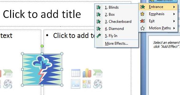
Powerpoint starts you out with a selection of templates as indicated below left. No doubt these will be useful in most cases but in the problem we will be doing these will not have much of an effect. In the middle is a super box that microsoft provides with the use of some of these templates. This superbox allows the user to insert bulleted text, tables, charts, clip art, movies and pictures. All of these objects can be inserted using the insert tab of the ribbon but this box makes it much easier. Finally, any object inserted can be animated. Animation gets you close to programming. You have the ability to create entrances and exits among other things. It's kind of fun and last term I concentrated on this with my classes. For our classes this term, it will be more chocolate and vanilla. Howver, below right, you can see an object and through the animation tab, the possibilities exist for entrance, exit and enhancement options
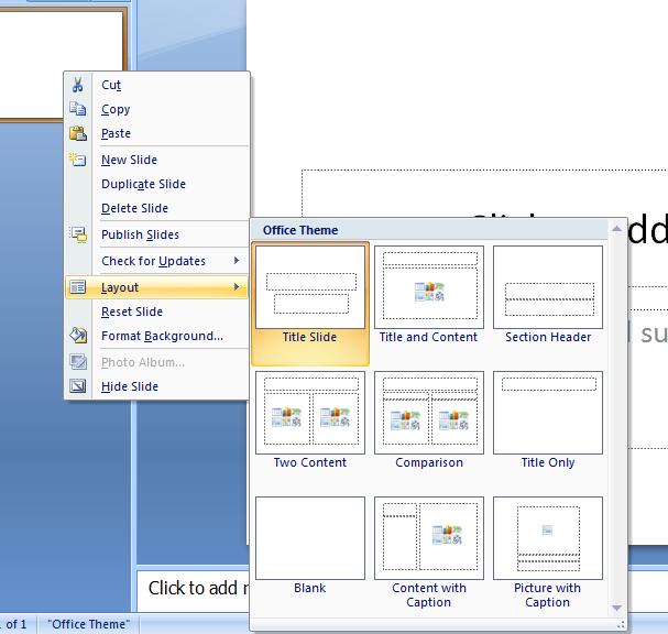
Let's open up powerpoint. Keep in mind, that this is to some degree Word without text. Text is very important, but it is part of objects. To the left is what is known as thumbnails which was pointed out in the lecture on Word but not used. It is situated where document map is located. As opposed to documents, Powerpoint works on slides and slides have one of 9 possible starting templates designated as layout which you can see by right clicking the thumbnail. One of these templates is blank. Below, is an example of this.
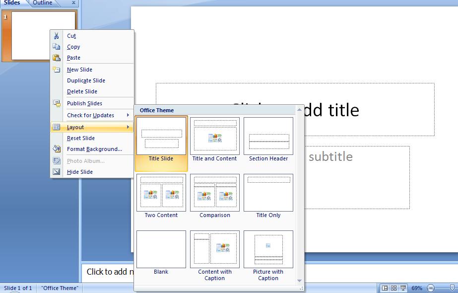
 Notice these templates are made up of text boxes and what Microsoft calls smart boxes. We will return to these shortly. But first, how about the background. For this, click design. If we had the time, we could have done this in Word as the coding and principals are applied. You will see 20 themes (including the default white) and click on one, Even with the default layout, you should be able to see a difference. Now, each of these themes can be modified and the preview tools used in word can be used here. Click on font and see how the whole slide is affected. Similarly with colors where a set of colors are indicated. You can if you want affect the underlying style by using options of background styles in essence to make your own type of theme. If you really get good at this, find a piece of the background and click your right button and you'll get more options for this as to the left.
Now, let's return to the templates themselves. You are familiar with text boxes in Word and windows but these text boxes have a bit if smartness associated with them. We should be dealing with the default template. One of the text boxes should say Click for title. Move your cursor inside and start typing CIS103. Notice that a certain height and justification is assumed (the justification is centered) automatically. You can change the font size if you wish, but in my case I am seeing an assumed 48 points.
Right below is the text box indicating click for subheader. Move inside this and type Section 181. Again, defaults are at work as far as centering and font size.
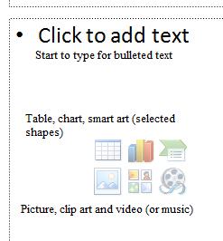
Let's alter the template to the most advanced possibility - this would be comparision. Click this and you will see that our text has been incorporated into the new template. Now, you have some added text boxes and we can assume that defaults as far as justification and font size are established for them. We, however, are interested in what Microsoft designates as a smart box and you can two of these. The smart handles 7 different functions. You can insert tables, charts, smart art, pictures, clip art or media (audio and/or visual). Not surprisingly these options are available to you on the insert tab of the ribbon except that it is more convenient to do these insertions through here. Now, surprisingly, we will ignore all of these. You will notice a seventh option, click to add text which we are about to do.
Start typing the microsoft office components we are to study in this class - Word, excel, powerpoint and access. Notice that these become bulleted as you type them.
This smart box has become a text box. What is a text box. It is a separate area from the word processing buffer (assuming we were in Word) where you can deposite text. Before going further in the discussion of text boxes, let's spend some time dealing with bullets and numbers in Powerpoint. It is similar to Word with several exceptions as you are in a text box. There is a verticle alignment feature which we can test amd, even more surprisingly, a text direction component. We touched on this when talking about drop cap ion Word but you can now see this in play here.
Similar to what we looked at in Word as far as pictures, text boxes are movable which we will demonstrate and you can affect their size. Notice that aspect is not a problem since each piece of text is defined with a font size.
Text boxes in Word and powerpoint can be inserted but there is a difference in Word versus powerpoint. In word, you define the height of a text box. In Powerpoint, your entry into the textbox defines the height. You define the width. As you create the text box, a format tab becomes available on the ribbon and you can see that this is similar to several tools we already studied. Take a look at the preset shape styles and the ability to make the text look like word art. You can even change the shape which your instructor wil ltry to do. What you can see here is that you can make a text box into an annotation and the other things we studied in Word. In fact this is what word does.
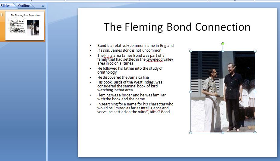
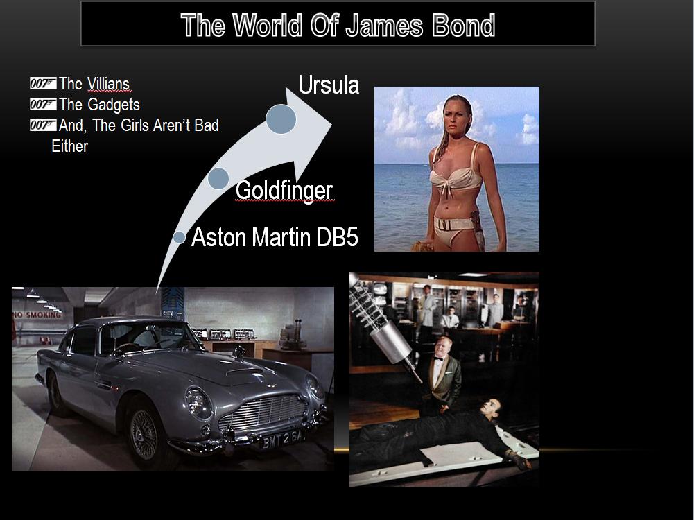
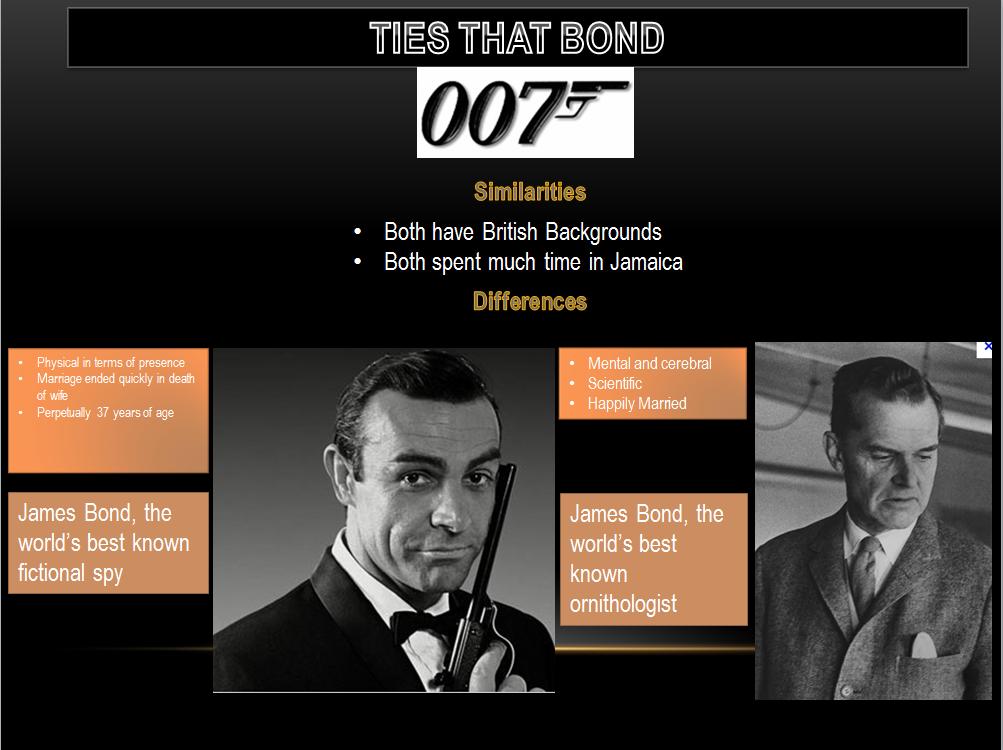
Now, let's deal with the second smart box and insert a picture. I know you will be shocked, but your instructor has been studying the life of a former very prominent Philadelphia area resident who wrote the famed book, Birds of the West Indies, in 1936, later reissued in 1948, 1960 and 1999 whose name is James Bond. Surely you also have read these books pertaining to ornithology. He was a very famous ornithologist and worked for the Academy of natural sciences. Of course, it's possible that you may have run across the name 'James Bond' in another capacity and, while your instructor doesn't think that this really is true, there are some that believe that an author used this name, given that the author was a birder and was familiar with these books, when he went on to write a set of books involving a character who dealt with espionage. You can access the Philadelphia, James Bond's, picture with that certain author, Ian Fleming, whom your instructor also studies by clicking here
Your instructor will kead you into the creation of a powerpoint slide as indicated below
For our final we want to crate a five(5) slide powerpoint presentation. Below is the 5 slides


The following are the files needed to create this. These are not exactly the pictures used in our examples but they will work.
007logo,gifOnce we have created this, we want to deal with movement of slides and animation. We are going to try to get the gunbarrel scene to act like the movies.
Click on transitions and you will see that on mouse click is checked. With this, you need to do something when a slide is appearing top move to the next slide. A mouse click or a hitting the key board will do this. Let's try this. Click from beginning on slide show as we show below.
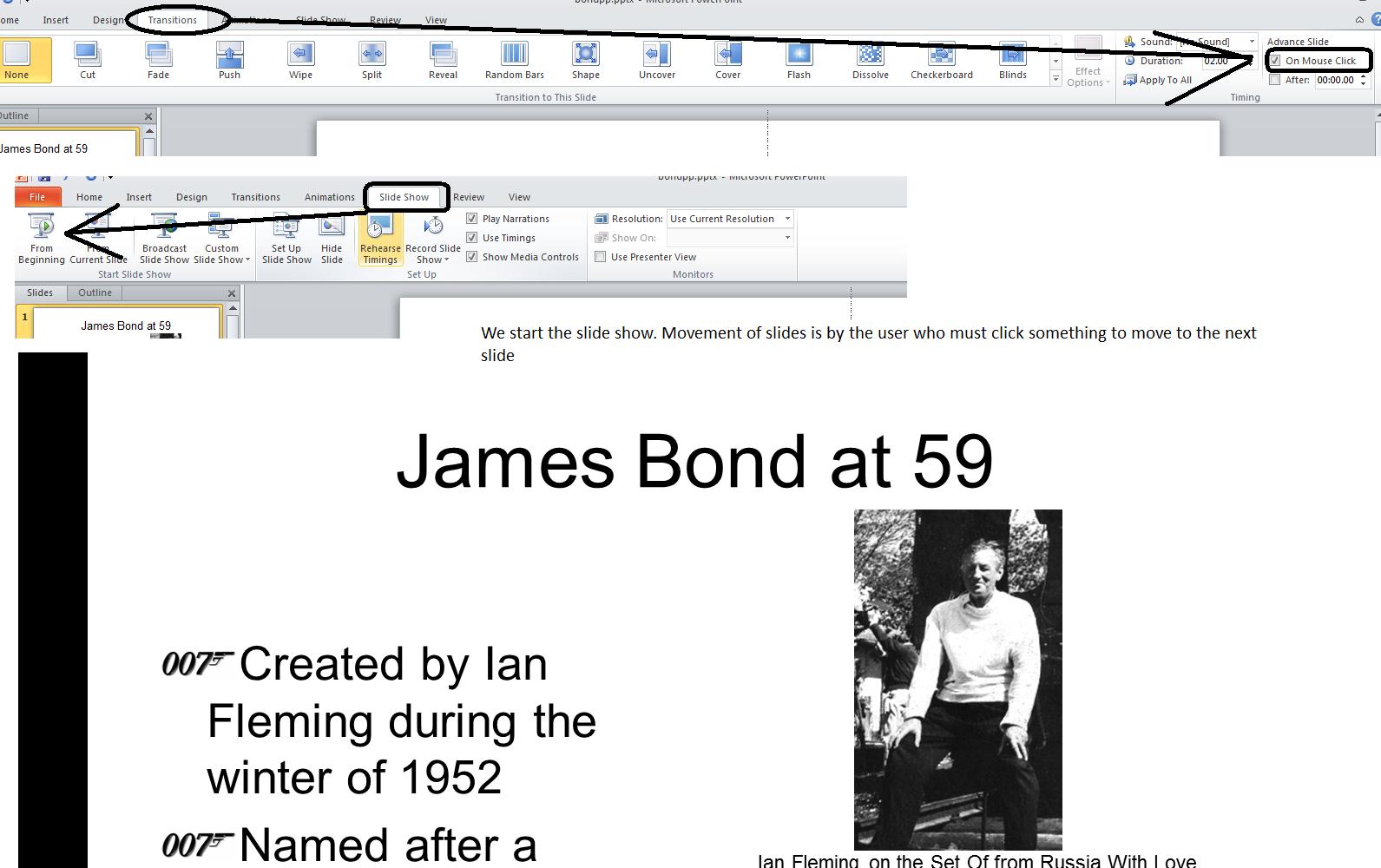
Let's assume that we want to have a transition as we move into the next slide. The transition tab handles this for us. Notice that transition is set to none. Click cut and then preview. Did you see a slight difference in the slide as it started up. Try wipe. you will notice that there is a specific transition. Click effect options and you can control from what location the wipe starts. There are many others that you can see broken down into subtle, exciting and dynamic. We'll try a few in class. But, wipe, has specific meaning to the content of this powerpoint slide show. Peter Hunt was the film editor of early James Bond movies and he was advised, if not urged, to spped up the move,ent of these films by Terrence Young, one of the early Bond film directors. Hunt's solution was what you are seeing as wipe. Movements in these movies were not done by traditional hollywood means but by this new technique that Hunt helped create.
Now, what if we want to time this show. On all except the last slide perhaps 5 seconds are needed to take in the slide. For the last slide, perhaps 10 seconds. Now, put in 00:05 (or click the spin control 5 times. Don't forget to unclick the on mouse click (although you can use this to transition faster, if needed). Now apply to all and you will see that all the slides are at 5 seconds. We can run this but we will notice that the last slide does not allow enough time to read. Set that slide to 10 seconds duration.
Before we start, several announcements: Your excel test will be on Monday, Dec 12th. This is an important test per this class. Not everyone did well in Word from my records, and perhaps only half of you submitted Access test takehomes. You want to be able to handle the Excel test in some manner. I would suggest studying your book, studying thid web site but adduing the tests that I have mad available clicking here. Thise who do not take the esxcel test wuill receive a 0. Any legitamate absenses will be handled (and grades modified) after classes are over and my grades are in.
After the excel test on Dec 12th, the course becomes split as we study Powerpoint. The Mon-wed class will have a lecture in powerpoint on Dec 14th. A one hour 'exem' will occur on Dec 19th. Tghe Mon-Fri will have both a lecture and test on Dec 19th as we extend the final time period an hour. As far as the Mon-Fri class, it appears I was wrong and we will be in the same room on Monday as usual. As you know, there is no projector support and we will have to do as best we can.
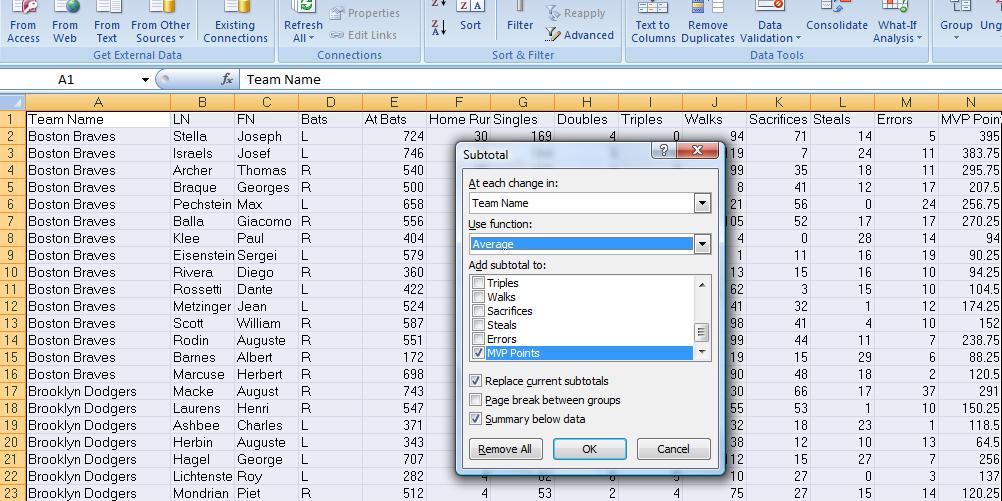
At the end of the last lecture, you will remember that we were dealing with the CBL. We had used the formula given in the write up to create a new column designated as MVP points and then sorted on Mvp points (ascending to descending) to find out the individual winner who is Joseph Stella with 395 total MVP points. We also sorted in descending order the column of home runs and found that both Stella and Auguste macke led the league with 30. Obviously, Stella has had a great year - a lot better than your instructor, we could add. Two columns were missing last we dealt with the excel workbook and I have rectified this and so you can load what we had by clicking here
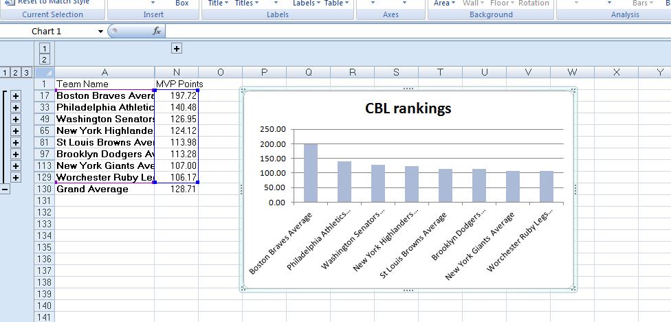
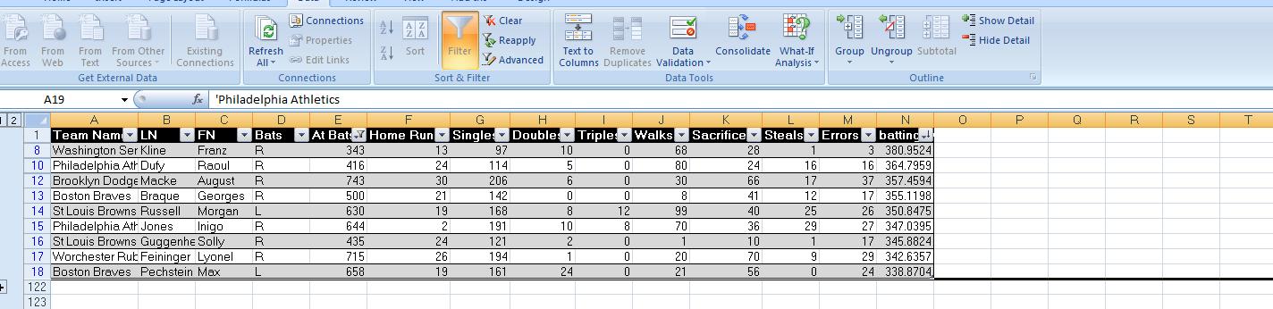
We are doing sheet1 by subtotal. Remember, in subtotals, you have to do the prep work. We want to find the average MVP points per team. Just like the previous problem where we needed to get the book titles together, we need to get the players of each team together. To do this, we need to sort on team name and it doesn't matter whether you do this ascending or descending. Once we have our sheet sorted, we move into subtotoals by clicking subtotal in the data ribbon. We are using breaks in the team name to do this. We need to select average and the column we need the info on is the last, MVP points, and that is already clicked. Below, you can see this.
Clicking on control 2 will just show the teams and their average points. Sort on points and you will find that the Boston Braves (who are now the Atlanta Braves by way of Milwaukee) are the winners. Format to two decimal places and compress columns B through M. Now, we only see columns A and N, Highlight the h3eader and team info (not the grand average info) and run a bar chart and you should have what is indicated below.
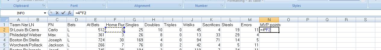
Onto the next sheet. Looks the same as when we started the first. This time, let's use excel to help with our formula. Home runs are in F2. Move your cursor to N1 and enter MVP points. Now into N2 and put =4*. Now click on F2 and you will notice an F2 is placed to the right of the * in N2. Below, we catch this. Notice that f2 is outlined (Microsoft terminology for perforations around a cell). This will be bordered in some color as we add the next operator, in this case a + for addition.
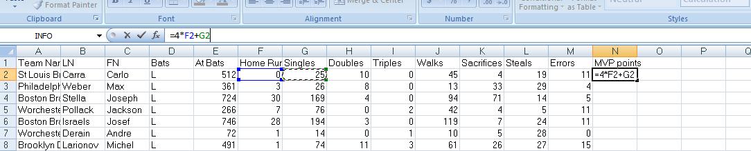
Now, let's finish this off. Having put in the + (notice the border around F2 has become a normal border), we click on g2 and g2 is now next to the + as n dicated below.
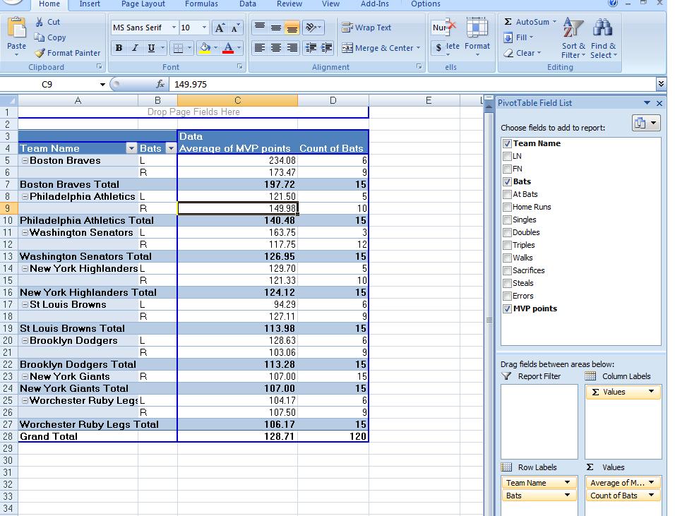
Let's finish this off to get the numbers we had in the first sheet. Remember that the first individual ends up with 57.5 and the last player is 290.5. This sheet is going to be done by pivot table. There is no prep. It's right into pivot tables and all we need to do is click inside the table and click the insert tab and then pivot table. Once into the pivot table, select team name and mvp points. Our results should look like subtotals. Through the pivot table, sort hightest to lowest, format to 2 decimals, graph and format the pivot table. Below, shows where we are at this point.
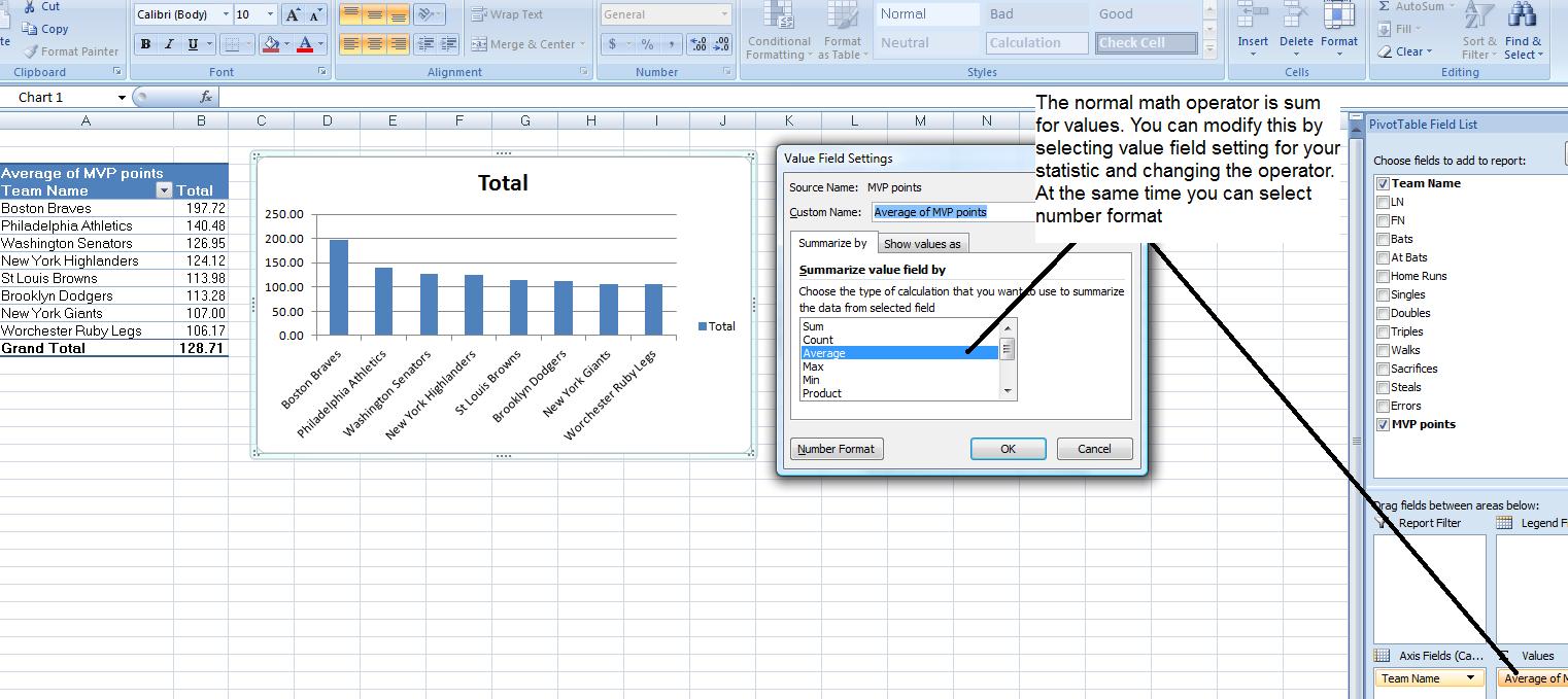
At thiws point, our pivot table looks like our subtotal info. I call this a 1-d pivot table. Let's see if we can show you something a little more complicated. Each player bats either right or left handed (we assume no switch hitters). Click bats and drag bats fvrom rows to columns as i will show you in class. Now, the pivot table is 2-D with rows and columns. You should be seeing something like the following.
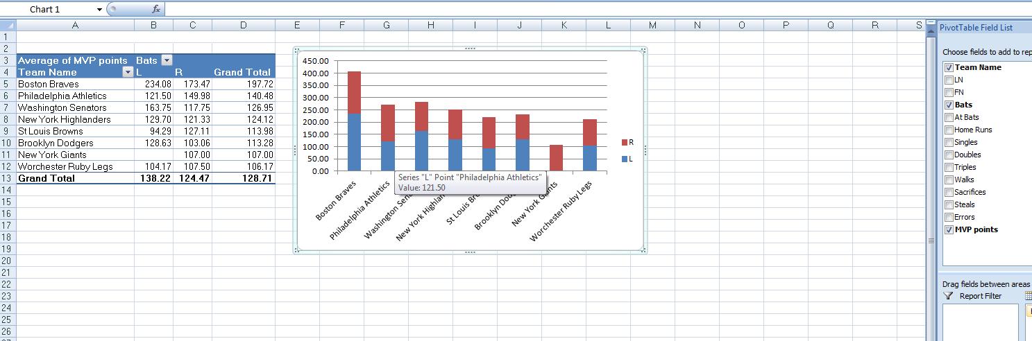
Notice the chart also. This is what is known as a stacked bar chart where two (or more) sources of info make up the bars. Pivot tables have tremendous capability which includes the ability to calculate information of the subtotal (group basis). This is similar to the having command in SQL. let's assume, given this information, that we would like to know the percentage of left handers on all the teams (it is possible that your instructor has picked left handed based on his own biases and you must always be aware that you may be adding such a bias in any statistic you try to determine. In this case, absolutely, your instructor has picked left handedness given that he is a natural left hander).
Now, to do this, we need to add a count here.Drag bats to the value box and since this is a text field, the system will automatically set this as a count. Cut the chart as it will now start providing meaningless information. You should see something like the foloowing.
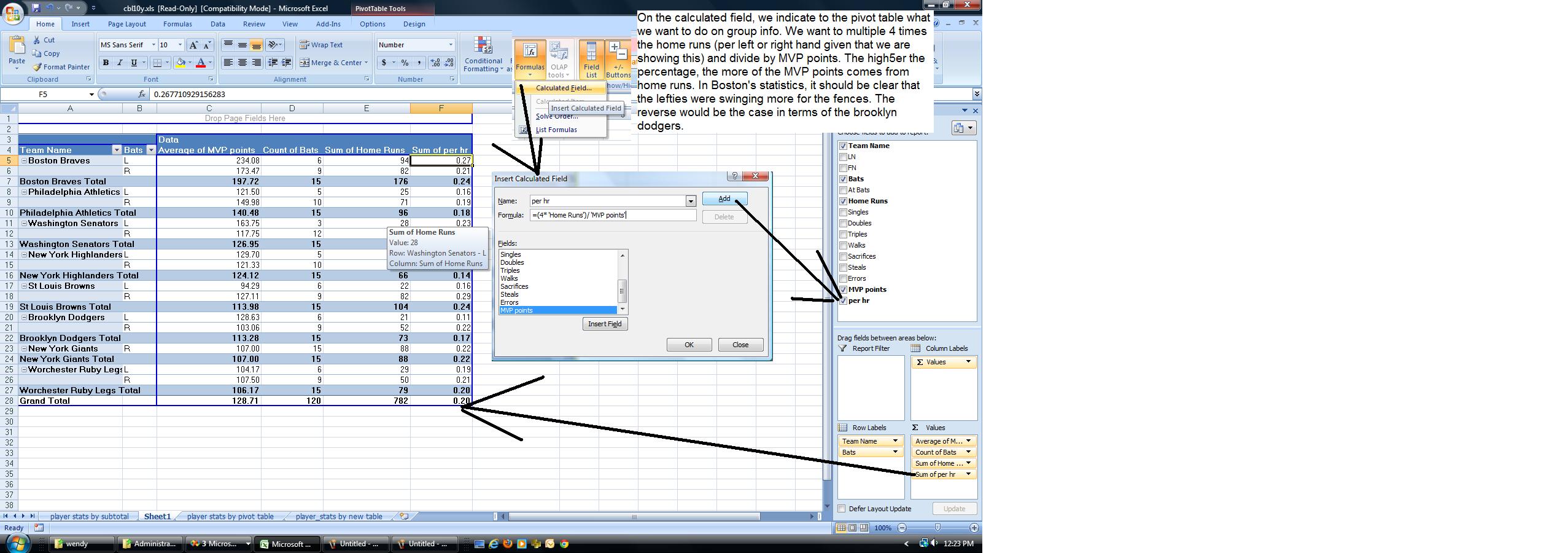
We want to calculate a field based on this info. We would like to know on a group basis by team, how much effect did the home runs have in mvp points as a percentage for left handers vs right handers. The higher the number, the more home runs influenced this. Add home runs to our values. This should come in as a sum. Now, there is a control designated as formulas. One of the options of formulas is calculated field. This works out math on a group basis. We are showing home runs and MVP points by left and right. Whatever we ask, it should show this by left and right. We are going to ask for 4 * home runs/ mvp points. Home runs and mvp points are already fields. we start by entering (4* after the equal sign. Click the field homeruns. Enter a slash (/). click mvp points. Above this call this field per hr and click add. Notice that this has been added to our list of fields. It should already be clicked, but if not, click it on. Do you see the percentages? Set this to 2 decimal places. Below, we follow this argument with a picture.
We turn our attention to the new table construct. Let's do this by formatting. On the home tab, select format as table. Pick whatever color you want. Before we do our calculations, let's determine several things here. Who were the top 10 home run hitters in the league. Click the home run column header control and click number filter. Now, ask for top ten. Below, we show the process.
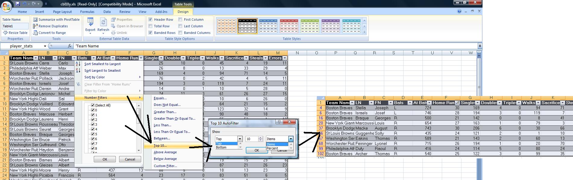
You can sort the home run column to see these in descending order. Now, let's answer another question not done before. Who are the top 10 players batting averages. Batting average is the number of hits (homers + singles + doubles + triples)/(at bats - sacrifices). Multiply this by 1000 and you get a set of numbers. In this column, sort descending. We will only look at players with 300 or more bats. Set this as a numeric filter in at bats. Now, back to batting average. Again set a numeric filter and select top ten. You will notice that only 2 show up. This is still considering the players with less than 300 at bats. In both access and excel, logical and really mean what they say. The way to handle this is allow the filter for 300 or more bats, sort batting average descending and then group player 11 through the end together and apply group by compress. Below, you see this.
 Move into N1 and indicate MVP points. N has been added to the table.
The new table construct (or whatever you want to call it) combines several ideas into one click, if you will. The old table auto format has been extended and allows you to tailor a layout design depending on whether you have a header, total column, want banding, etc. Once a total column is insicated, an additional row is generated automatically for the totals replacing autosum. Calculations done in the first line item (row 2 in our case) are immediately copied down although this can be changed, but we will not do this in class. Automatically, every column name gets an additonal control allowing for sorting on that column and for filtering knocking out the individual need for these controls for the most part (although understand that your instructor could complicate any problem to he point that you would need a more advanced sorting capacity supplied on the data tab).
What do you lose with this new table construct? You cannot subtotal since the emphasize is primarily on a pivot table at that point. However, if I get a chance, I will show you how you can take several aspects of subtotals and use them in the table construct. You can access the file as we left it by clicking here.
 There is a little prep work on your point if you wish to do this or you can use other controls to resolve need for additonal columns. We've done this enough that I will show you two ways to deal with. We know in this problem we need to calculate the profit per line item. We can make provision for this in 3 ways. The first is to specifically designate another column. In this problem, in the insert tab, click table and you see what's on the right. Now, instead of =$A$1:$G$113, change that to =$A$1:$H$113 and when the table is situated there will be a last column, designated as column1 where column H is. Below is the final result of thisd and this is what you should be seeing at this point.

Now, for a second situation. let's undo, and repeat the process, but this time no changes to width. You will create the new table construct using A1 to g113. Now with the table set, move to the design tab on the ribbon and click resize table. Back comes the range indication and we can change this as done previously. Below, you can see this in action and when you change the G to H, you will see the results of what we had done before.

Now, let's undo again, so we still have the new table construct but going fron A to G. Now direct yourself to G113 which at the moment is the last cell in the new table construct. Right there is the handle but there is a slight addition (although you might need a magnifying glass to see it). Mocve your cursor to the handle and not surprisingly the crosshair shows up but nudged the mouse slightly in cell g113 and a 135% grabber will appear. You can use this to add (or decrease) the size of the table construt as will be shown in class.
We have one more thing to show you about setting up the new table construct. All the things we've done today pertain to formatting and in the case of formatting, all the undos will work. Undo everything to the point where we forst looked at the fourth sheet. A quicker way of inserting a table construct is on the home ribbon. Click format as table and you can choose the design type to go with your new construct. I like this better since it knocks out the default design type instituted with the table button on the insert tab of the ribbon. Below, you will see that are starting the process. Pick a layout you like and make provision for a new column as we have described above.

With our column1 in H1, let's change this to profit. Now, another change that we can see is the type of reference. In prevuious situations you could point to a cell and its deignation would be applied. Now, pointing gives you a designation per the table. Below, we are using Excel's pointing capacity to set up our formula.

You should have noticed that calculations are automatically being copied down through the colun. This is also a great feature since 99% of the time this is what you wanted to do anyway. But, what if this is the 1% of the time that you have a spreadsheet that you do not want to have this occur. You can turn this feature off in excel using the contriol that appears after this takes place. I don't know what this control is called but below is how to turn this autocalc feature off.

In previous versions of excel, there were always problems between setting up a row of sums (using autosum or just applying the sum function) and how the rest of excel ran. In fact, in one class at Penn State, I spent a week showing where autosum could or could not be applied. This has been resolved through this new table construct. Click total row in the design tab. Besides affecting your options per layout, look at the bottom. A new row 114 has appeared and sum is a default for the last column. You can apply relationships to add to this sum or use ther control that appears once you have entered a cell on this row. Below, I'm in the process of adding a column sum for books distributed. I have entered the cell and on the control associated with this, I am entering sum.

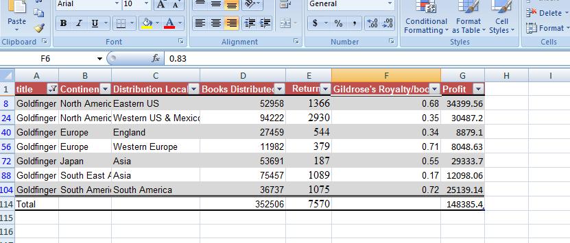
Let's verify sorting and filtering. Click the control next to title. Sort alphabetically each way. You can sort on color although in this problem I'm not sure what that would get you. Now, clikc for only Casino Royale. See how only those books show up. Look at the total sums. They are only set for Casini royale. This is a great feature and in many cases resilves the need for subtotal because in essence that is what you are doing only being specific as to what to show. below, since we used a poster of Goldfinger above, I've shown you the figures for that book.
The only advanced approach to summarizing data in the new table construct is by pivot table. Now, you could use the insert tab as we did before but sums might be added if sums were appearing as they are now. However, the design ribbon has summerize with pivot table and this possibility is already taken into consideration. let's run a pivot table on this doing everything we did before including sort, layout and chart.
We are about to do something in the pivot table that has been enhanced with this version of Excel and that is a calculated field. The calculation work on summation amounts and cannot affect the underlying table that created the pivot table. Let;s assume on this pivot table we would like to add a column for each book designated and meaning books distributed per month. This is books distributed divided by 12 and we will call this monthly books dist.
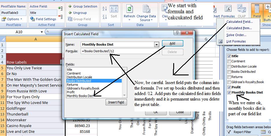
We now have a calculated field that is the monthly books distributed. The system generally defaults in this and puts the caluclated field into the pivot table. You can modify this default and if need be turn it off from appearing. Below, wee have finalized our pivot table.

Let's do another problem. Open up the documentation for the CBL. The excel spreadsheet is found by clicking here. Now, Let's do this problem similar to the Fleming problem by first using subtotals. But, we'll just move into the new table construct and resolve it by a pivot table. But, there seems to be a problem here as only one spreadsheet is appearing.
In previous versions, 256 sheets were available for each work book and there is no reason to assume otherwise in this version. In previous versions, the initial amount of sheets visible was an option. The same occurs here as the number of spreadsheets available to a new workbook can be modified although the default is 3. There is no default for existing workbooks and that is the case here. This excel spreadsheet was created from CSV (comma separated values or comma delimited) file which defaults to 1 worksheet when opened in excel. We can, however, modify this by inserting a new worksheet. Move your cursor over the player stats designation and click the right button. You now have several options. Choose insert and worksheet and a new worksheet is inserted before the one you are on. It should be designated as sheet1. Now, move your cursor over sheet1 and press the right button. Use rename to change sheet1 to player stats by table. By the way, by grabbing the sheet and 'lifting it', you can change the order of the sheets.
Now finally, let's copy the info from player stats to player stats by table. We'll use a trick to do this. You may notice that every time we do subtotals or pivot table or other things the system has the ability to determine the extent of the table. We can do the same. Move inside a table and click ctrl, shift 8. Notice that the table is highlighted (and, in fact, additional info may be available at the bottom of the screen). Now, to create the same info on the next sheet, use copy and paste. Copy the cells: move to the next sheets and apply paste. Now, we can attack this problem 2 ways: by subtotal and the new table construct.
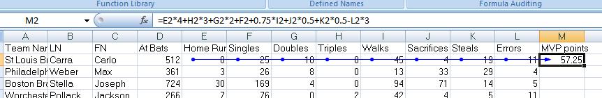
Let's work on the fist of these designated as player_stats and by subtotals. For this we will handle only the most home runs, the highest MVP points and the winner of the prestigious Rauer cup. As with the fleming problem, the first thing we have to do is the calculation for each line item -in this case for MVP points. The problem states that each homer is worth 4 points, triples 3, doubles 2, singles are 1, walks are .75. sacrifices and steals are .5 and errors are counted as -3. Let's set that in as a formula as can be seen below

Now, before we go further, over the years excel has added auditing features to the spreadsheet which you can find on the formula ribbon. We did this in the previous problem so this is a review. Click trace precedents and you will see an attempt to tie information together as a line with nodes in each cell used points to the resultant cell, in this case m2. To turn this off, use remove arrows. Below, we see the spreadsheet with trace precedents turned on.
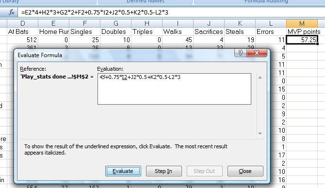 For the novice (and perhaps even the accomplished Excel spreadsheet user) this is an effective way of determining that all the cells needed in the calculation have been used. Remove arrow will end this and you can click that now. To see the formula in a dialog box and watch it calculate serially, click the evaluate formula. Each click of the evaluate button does a calculation and step in shows you the results at that time. This is useful for involved formulas where you are not resolving a problem as you think it should be formulated. This will show you the order of the calculations (this goes back to the precedence order of the mathematical operators) and might give you some insight to what is going wrong. To see all the formulas on the spreadsheet as one time, click show formaulas. To the right is the evalute formula in action. We have stopped it as it is about to calculate the walks part of the MVP points.
Now, let's continue with this problem. Using the double click as discussed in a previous session or copying down, let's fill out the column so that we determine the MVP points for each player.
We can continue with this problem by clicking here
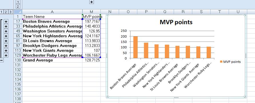
we know, by looking at the documentation, that the player MVP is that player with the highest MVP for the year. We can calculate this pretty easily now by sorting the MVP points column in decreasing order. When you do this you will see that Joseph Stella is our MVP player of the year. How about for the teams in general. Standings are defined as by highest average MVP points. We can do this in subtotals by sorting on team, and setting up for a subtotal on MVP points. Below we can see this in operation.

In essence, now, we are doing the same steps as the Fleming problem to finish this. Click control 2 at the right to see the subtotals per team. Sort the MVP points by descending order to get standing (remember that Excel handles the detail info by moving it with each subtotaled entry as you sort). If you want, you can group out all the columns between the team name and team MVP points. Create a bar (column) graph to show the results visually. Below, we see the final results.
We will do this problem by table construct using sheet2 (which we renamed above). So, let's click in sheet2. In the Fleming problem I told you what parameters to use for establishing the table extents. For this problem we will use Excel's tools to do so. We start with the list of the players as before. In the previous usage of this new table construct, we used the tab insert and the option of table. This time, let's do it a little faster. In the home ribbon, let's click format as ribbon and select a format. Anyone will do and your instructor will allow you to determine which one you want. The same info is asked of you as before, what is the extant, and the system assumes that you have column headers. Let me again remind you that for most of the things we are doing, it is important to have column headers and this class makes that assumption.
Let's start with the top 10 home run hitters in the league. Filtering is now set on and we can use this. We would like to determine the top 10 home run hitters. It could just as easily be the bottom 10 home run hitters: or the top 10% of home run hitters. We are entering the world of SQL, relational database theory. In one of the prior SQL conventions, top 10 and bottom 10 were defined. Excel meets this standard through filtering. At the Home Run column header. click the control and then click number filter. If this was a text column, number filter would be replaced by text filters. There are many options available here, some we may discuss. But, below, you should see the top 10 items.

 Choose this option and you will see what is indicated to the right. In class, we'll try a few possibilities but notice that these are not sorted: you asked the system for the top 10 and it showed but you have no guarantee that the top 10 are in order. We can resolve that easily by sorting just these 10 entries. In class, we'll extend this to look at the lowest 10, the top 10% (which for 120 players should display 12 entries) and the lowest 10%. But, another factor comes into play: what if we wanted to see these players numbers visually once we take off the filter. You can do this to some degree by conditional formatting which is very interesting and has been drastically improved in this version. Now, we'll take a subset of this and select green pennant flags for the top 10 home run hitters. Go to the home ribbon and click conditional formatting. Select new rule and choose only top or bottom. As our example, choose top 10 and set the coloring to blue. Below, you can see a composite of this result. By the way, the conditional formating can be used independent of the new table construct and is being used here to show the flexibility of working with excel

 Now, we need to create several new columns. One is for MVP points and the other for average. Both are defined in the handout and the link indicated above. TYo do this we need 2 new columns and this can be done in 2 ways. One way is to click the table design ribbon and then resize table. In essence this is what we did in the fleming problem. You would indicate changes to size of the table per column indicators. Another way, what we will do here, is to make use of a new indicator native to this table which can be manipulated. The picture to the right is an attempt to show this by graphics although it is easier to see and do in class. By this technique we will create 2 new columns. The first new column should be designated as Batting average, the second as MVP points. We'll work on batting average first.
Batting average is defined as the number of hits devided by the legal at bats. Hits would be singles added to doubles added to triples added to homeruns. Legal at bats are atbats - sacifices - walks. For each player we are talking about (using column notation) (e+f+g+h)/(d-i-j). For the player on row 2. the formula is (e2+f2+g2+h2)/(d2-i2-j2). Are all these parenthesis needed?. Could we do this in an easier way. Probably not! Remember we have to tell excel the order to do these calculations and the parends are probably necessary given the differences in priority of operation for the pluses and minuses versus the divisions.
Now, we've seen this before. Excel copies this formula down. Now, let's use the table with all it's capabilities. Although not asked, could you quickly indicate the average batting average for a player in this league. You should be able to answer yes to this. Remember, part of formatting includes the total row. Click the total row button in table style options and then at that row for the batting average column, indicate average. Below, you can see this done.

 Now, similar to the home run problem, let's determine the 10 best averages. In doing so, let's conditional format so these average show up in green. This is similar to what we did above with home run. But, let's extend filtering. What if we wanted to see the players whose batting average is greater that the average for the league. This is numerical filtering. Now, releasing the filter for top 10 in batting average, let's use the greater than or equal filter with the number .239 (which should be the average. We can see this operation to the right. The result should be those players who average is above or equal to .239. And, in doing this, notice that the excel spreadsheet gives you the average of those whose average is above .239. It is considerably higher at this point.
We've gone about as far as can with batting average. Let's calculate MVP points for each player. Above we have done this and the only difference here is the automatic copy down in effect. Now, again we can use our filtering or sorting capability to determine the MVP player winner - the player with the highest MVP points.
We are ready for the pivot table which we can invoke with summerize by pivot table. I've run out of time in documenting this here, but we will use a pivot table to determine the league winner. This procedure is a one - dimensional pivot table as indicated above. We will move this to two dimension using the left vs right handed batting as the next dimension. We'll play with this a little bit and then deal with a calculated field. What is the average batting average for each team. Above, outside of class, I did this for the fleming problem which you can see above. We will, in essence, duplicate this with this problem by using group numbers to calculate this for each team.
You don't need vast amounts of calculations to do problems using pivot tables. There is a problem that has been done in the last two tests which we could discuss now. Load the 777rauer statistics raw.xlsx file. We will use this file for the purposes of determining group averages. We'll do it by subtotals and by pivot tables. We are aiming at average kilobyte usage for each visit during the months of Sept, Oct and Nov.
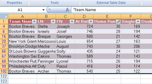
On Monday, we started the books of Ian Fleming problem. We created column g. I have set up a spreadsheet for you with column G filled in which you can access by clicking here. Because we are going to do this problem 3 ways, I have also loaded sheet2 and sheet3 with the entire table you saw in the word document. Please remember that there are 113 rows. The first row is the column header meaning that 112 of these rows are line items. There are 16 books and you will notice that they repeat 7 times each (16*7=112) and our assignment is to determine the profitability world wide for each book and worldwide for all the books.
Let's begin by renaming the sheets. Sheet1 will be designated as subtotal. Sheet2 will be designated as pivot table. Sheet3 as table construct. Now, move back to sheet2, Pivot table. For all the sheets, we start the same. We need to calculate the net profit per book title per book distribution point - each line item - and we can do this in the pivot table sheet. Our calculation should be (books distributed - books returned) * Gildrose royalty per book - books returned * .5. Set this up in this spreadsheet.
Now, for a one-dimentional approach to this problem, let's take a very simplified problerm and look at what tab operators would do 90 years ago to resolve this problem. Below is our accounts for a hyposthetical bank:
NY      200     M
NY      300     F
NJ      100     M
NJ      200     F
NJ      300     M
PA      300     F
PA      100     M
We start the process by sorting on sex. We have two possibilities, ascending or descending. If ascending, we see these accounts as F to M. If descending, M to F. Least line of resistance is ascending. When sorting, different algorithms are used to sort and collate info together. You have no guarantee of positioning beyond what you ask. In this case, if we were to use Excel's sorting, the only thing guaranteed is that the F are together as are the M's.
Whatever algorithm we are using, below is what we wind up with as we attempt to congregate Fs and Ms
NY      300     F
NJ      200     F
PA      300     F
NY      200     M
NJ      100     M
NJ      300     M
PA      100     M
Now, whatever technique or software that would be used, it would work this way. There would be two accumulations, one for subtotal, the other for grandtotal. At a break in sex - break indicating change or end of data - the subtotal would be printed and the subtotal counter set back to 0.
                        Subtotal counter    Grandtotal Counter  Print
NY      300     F           300                 300
NJ      200     F           500                 500
PA      300     F           800                 800
                    Break     0                         F       800
NY      200     M           200                1000
NJ      100     M           300                1100
NJ      300     M           600                1400
PA      100     M           700                1500
                    Break(Eof)0                1500     M       700
                                                  0     Total  1500
Let's look at this by state instead of sex. Below is our accounts:
NY      200     M
NY      300     F
NJ      100     M
NJ      200     F
NJ      300     M
PA      300     F
PA      100     M
We start the process by sorting ascending on state.
NJ      100     M
NJ      200     F
NJ      300     M
NY      300     F
NY      200     M
PA      300     F
PA      100     M
Again, whatever technique or software that would be used, it would work this way. There would be two accumulations, one for subtotal, the other for grandtotal. At a break in state causes a subtotal.
                        Subtotal counter    Grandtotal Counter  Print
NJ      100     M           100                     100
NJ      200     F           300                     300
NJ      300     M           600                     600
                    Break     0                             NJ 600
NY      300     F           300                     900
NY      200     M           500                    1100
                    Break     0                             NY 500
PA      300     F           300                    1400
PA      100     M           400                    1500
                    Break     0                             PA 400
                    Break                                                  0     Total  1500
Now, let's do the same for this problem of the books of Ian Fleming. We need to congregate all the casino royals together, all the goldfingers. We should sort on the book title. Now, one note. In a previous sort we used the full scale sort icon given that another line item was added for totals. We will not have to do that here. So, we can use the simple sort A to Z or Z to A that we have seen on the Data tab of the ribbon.
Move your cursor anywhere on the first column of books. In fact, we'll split this up so that we will all see the same result even though we start from a different place. Click a to z. below is a composite of the result.

Notice hte grouping of the titles. We are almost done. We need the system to give us subtotals on these grouped titles. The data ribbon provides a tool for this which you can see far right. This is sub totals and clicking it produces the dialog box described below. Note, however, that if you set your table ot the new table construct, subtotal is grayed out since the new table construct gives you many of the eatures of subtotal and much more.

Clicking yes adds a set of rows to your spradsheet. Every subtotal is added as is a grand total. In our case, there are 16 books and a grand total giving 17 new rows. In additon, a set of controls are instituted to the left. Below we see part of the spreadsheet after clicking yes to subtotals.
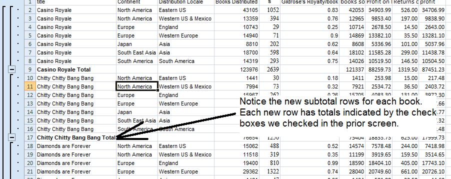
Look on the left at the controls. Notice that there are 3 of these (1,2,3) at the top. 3 is detail and subtotal info. 1 is just grand total info and 2 is what we want: subtotal only info as indicated below. Notice grand total info is also included. Columns which are not used for breaking or for totalling appear unpopulated. You could group these and, in essence, hide them from view. Anyway, below is our subtotalled info.

Excel treats cells that are grouped out of view as not part of the spreadsheet when selecting. This is true in terms of sorting. There are 130 rows. In view, there are 18 at the moment. The first row is the header row, and then we have 16 rows of subtotal info and then the last row, grand totals. In a previous situation, we tried to sort with totals and totals moved through the spreadsheet. With subtotal, the system knows that grand total should be at the bottom. We would like to sort these titles on the basis of profitability - the highest at the top to the lowest. Move your cursor anywhere on the last column and click z to a in the data tab.

Now, the same principle applies to graphs. let's do a bar/column chart on the books and their respective totals worldwide. Highlight the books (except for grand total) in column A (in essence the first 17 of the rows shown) and likewise use your control key to add the first 17 cells of column J. Use the insert tab of the ribbon to create a bar chart. Below, I've gone a little further by setting an angle for the descriptors. The principle is similar to the other time we sloped text. Move your cursor on the titles and click your right button and select format axis. You will see the more modern version of the dialog box we had seen in the previous example. Click alignment and set 45 as the degrees in custom angle.
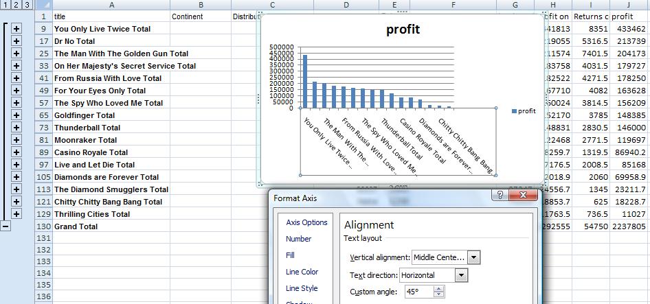
Now, a 2D approach looks at this data and determines all the possibilities of the columns in question. Here for sex, the possibilities are M and F, for state the possibilities are NJ, Ny and PA. Below we see the possibilities before doing any math.
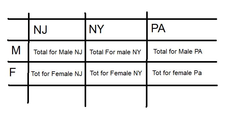
Now the procedure would be to run through the list and add the account balance to the appropriate cell. In the first line item, we are dealing with a NY female. We would add 300 to the cell at Row 2, column 2. Suince it is initailized to 0 at the start we now have 300. If a 100 had already been there, our total would have been 400, instead.
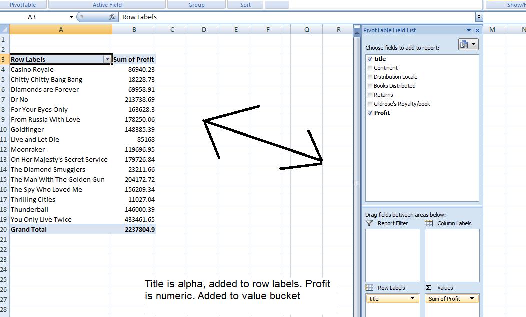
In the pivot table spreadsheet what are the possibilities to the problem. The family wants to know the profitability per book title world wide. This is a 1D problem, but we will be using a pivot table to resolve this. What do we expect as the titles of the row in the table that will be built. It should be the book titles. What should we expect in the cells of the table. Each book title encountered adds to the total for that book title that had already been accumulated.
We start the process by clicking thr Pivot Table control in the insert tab of the ribbon. Thhis should give you the limits of the table. Note. Pivot tables need column headers to work. If a column does not have a header it will either not be included or the pivot table will fail. We have designated our new column (for line item profit) as profit. Although there is no requirement, put the pivot table on a new spreadsheet (this is the default). When the pivot table appears, click title as indicated below. Notice at this point, we have listed the book titles in sequential order and the designation title is in row labels. That's exactly where we are at.

Now, we are looking for aggregate profit per book. Click profit and you will see the pivot table below. By the way, this is not magic. Book title is obviously a text column so when clicking such a column, the system added the designation to the row label bucket. Profit is a mathematical column. Math columns get added to the values (in previous versions designated as data) bucket as you see.
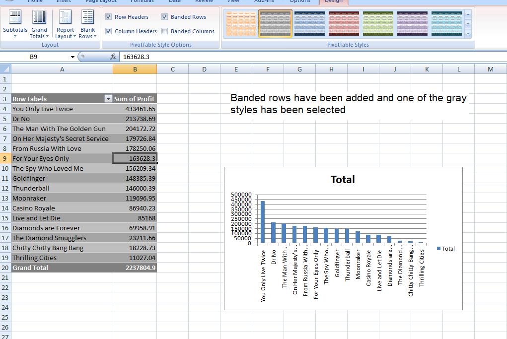
These books are already sorted by name. Probably, the family would like to see the titles sorted in descending order for profit. Your pivot table provides tabs that support its operations. One of which is sort. Look at that section, move your cursor anywhere on the column representing profity and click z to a. Below we see the result.

You know that we can chart in Excel. Charts also exist as far as pivot tables are concerned. Again a bar chart is the best for this problem. Again, look at the pivot table tab. Chart is an option. Click that and select column chart type. A pivot chart is produced with more capability than previously seen. This added capability is geared to turning on or off the charting of different titles.

You have formatting options to this pivot table also. Click back onto the pivot table and click the design tab. I have added to this by clicking banding row and selected a gray (some say to go with my personality) format. Below we see the result.
As promised, we are about to deal with detauil info, sum that up into subtotal info, then deal with this subtotaled info for an answer. You can look at this in one D, or in Two D, For Two D (and above) we have 2 possibilities: Pivot tables and the new table constrcut breaking down into pivot tables.
Before returning to subtotals, let's show you a taste of 2D. Move your cursor to continent and drag that into column labels. Once done with that, click in the chart and request a stacked bar chart and you can get the following.

We had done the beginning parts of the Big W problem. If we wanted to, we could delve into a large set of spreadsheert mathematics. Instead of that, I want to show you an extension of the problem using absolute addressing and the if statement. Absolute address, designated as $C$R, is what most of you thought excel addressing to be as we started. By designating $c$r, this never changes as we fill. Look at the difference between this and relative address. The row designation changes as we fill down (or the column changes as we fill across).
The if function is a very important for doing more sophisitcated excel spreadsheets. If uses the results (or data) on a spreadsheet to determine what to do. It's syntax is =if(condition, true, false). Now, condition is a test. Using operators such as < (less than) < (greater than) = (equal) <= (less than or equal) >= (greater than or equal) and <> (not equal) we can test the condition of cells (or just a cell). In Truem we can place a value to display is the conditon is true. If false we can place a value if the condition is false. =if(b2=$b$11,1,0) is such a case and this is acombination of if and absolute address. if b2 is equal to b11, place a 1 in the cell where the if statement resides otherwise place a 0. Copying this down (filling) would give =if(b3=$b$11,1,0) - notice that b2 has morphed into b3 but $b$11 stays as $b$11
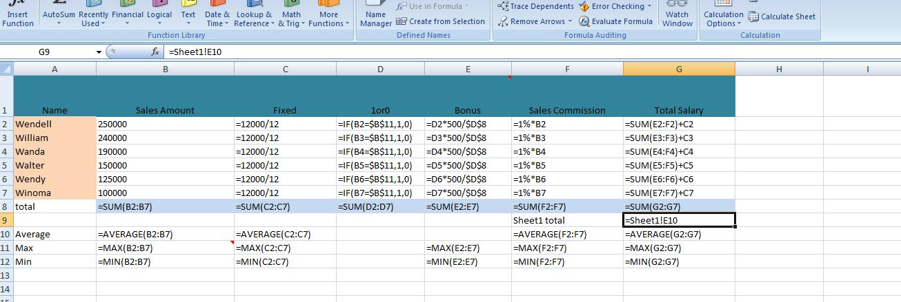
Let's finish this problem. click here to load this. We have copied the cells in sheet1 into sheet2 and we will do our work in sheet2. We have added a new column as D. We indicate the title as bonus as you can see
In sheet 2, lets add a new column D (inserting a new column at D). Call this column 0or1. Use the if statement to determine if the represetative value in column B is the max. We can do this by using =if(b2=$b$11,1,0) as indicated above. Fill this down. We use b3,b4,b5,b6,b7,b8 but are always comparing against b11 (in this case $b$11). 1's will show up where the corresponding column b equals $b$11, 0 otherwise. If b9, sum this up. If one winner, a 1 will appear. if 2 winners (a tie) a 2 will appear and so forth. Now, look at column E, the bonus. The calculation =d2*500/$d$9 should provide the monetary bonus for us and will give the correct bonus in case of ties, three winners etc. We will have ot modify our total salary as will be shown in class. Below, is the formulas for doing this.
Onto our next problem. The major flaw of this problem is lack of detail info. We, in essence, have summary info for all the sales paeople. Life, and especially, data processing, is not like this anymore. You use excel today to break down detail info into summary info. The rest of our study of exc el will be to do this. There will be three techniques. The first one, subtotals, we will do just one time to show you an older way of handling this. After that, it is dealing with pivot tables and pivoot tables through the new construct table which i think you will like.
Our first foray into this is one of my favorite problems. The books of Ian Fleming. There is no excel spreadsheet. We have to create and there are 113 row (112 line items) of information. And, we have to work out some calculations. Calculations seem to be a problem for most students in this school. We will do this correctly in class but keep in mind that on the test, you do as best you can but you must make sure you finish the problem so that I can give you the highest amount of credit.
Onto our first problem dealing with detail info into summary components. Click here to load a Word document indicating the books of Ian Fleming. In all of these problems, it is important to read the problem carefully. In this one, the heirs would like to know the total profitability of the books and the profitability of each book. Notice that each book title occurs 7 times. We need to be able to sum up the profit of each book into a total.
>p>First, what is the profitability per line item. At that time, books go to a book store. If sold, there is a price per book that goes back to the publisher (in this case the heirs). returns are not sales. And, it has been agreed that each book returned will cost the heirs 50 cents. In class we will indicate the formaula but first we must copy all the line items into excel and we will show you how to do this in class.We can access where we left off on Wednesday/Friday by clicking here.
We were in the midst of formatting and I have chosen currency, 2 decimal points and separators. Notice that our sales total is a set of pound signs. This brings us into another distinction between text and value (numbers). Text, besides being right justified, will bleed into the next cell to the right (and it could be several). This assumes that nothing is in this right cell. Once data is put into the right cell, the text is truncated in terms of view. Note: The text still remains as an entry in the original cell. Nothing is changed as to this.
Value (number) works differently. If there is not enough room to display (with or without formating), pound signs replace the value. Note again: Even if pound signs appear, the math still works and you can reference this cell in mathematical equations.
To resolve the pound signs, we need to manipulate the width of the column. This can be done by grabbing the point between the column header designations and manipulating the width or by double clicking this separator and the system will apply auto width which polls the entries in the column and sets the width of the column to the largest entry.
Now, let's set some column headers for this spreadsheet. The term column header pertains to text that is top most for each column that describes it. In addition, we would like to enter a title and in excel titles are text in a cell which is the result of the meerger of several cells.
We are going to look at insertion. This can be done on many levels including insertion of a cell, a range, a row and a column. Unless you are at the row and column level, a second question is asked of you. Are you moving down the other cells by rows or by columns. You are not asked this question when a row or column is inserted. In additon, there are two ways of requesting insert. The one not recommended by me is the formal approach using the insert control on the home tab as indicated below.
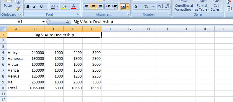
In the case of an insertion of a row (or column) to use the context sensitive popup using the right click of the mouse. To do this, click the row that will move down when the new row is inserted. In the case of several rows being inserted at the same time, drag your mouse and select the number of rows where the first row will move down. In our example we need to add 3 rows. One for the title of the table, a blank and then the column header. Below, you see the start of this, Rows 1 to 3 are highlighted. A right click has made the pop up menu appear and we are about to click insert on that menu.
We can handle the title first and it can be as simple as the Big V Auto Dealership. We want this to center over our table. Insert Big V Auto Dealership in A1. It will bbleedc into b1 abd probably c1. Highlight the range a1:e1 and click the merge and center button in the alignment group of the home tab. What we've done here (as mentioned on Wednesday in class) is create a large A1 spanning to F1. And our result should look similar ot what we show below.
Now, we will allow the blank row to stay at row 2 as it is but now let's concentrate on the header row which we will put in row 3. Each cell of row 3 will provide header info for that column. But it's not going to look good as we first put it in. We will have to manipulate the row as you will see. But first, let's enter the info. Column A is Sales Person. Notice how it bleeds into the next cell. That next cell should be Sales Amount. Column C is fixed. Column D is sales Commission. And, finally, column E is total Salary.
One solution would be to widen the columns as demonstrated on Wednesday. While it will work, it will make the spreadsheet look odd with the columns being to big. WHat we would like to do is have the system break the cells so that there may be multi-leveled descriptions. And that's what we are going to do. But first, let's bolden these descriptions and increase the point size. With row 1 selected (and this is done by clicking in the descriptor of row 1 where it says 1), increase the point size to 12 and click the bold button.
Now, you have two choices as to selection. You can use the pop up menu as we have done before and select format cells or the format control on the home tab and select format vcells. Below we show both possibilities.
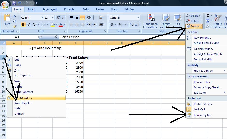
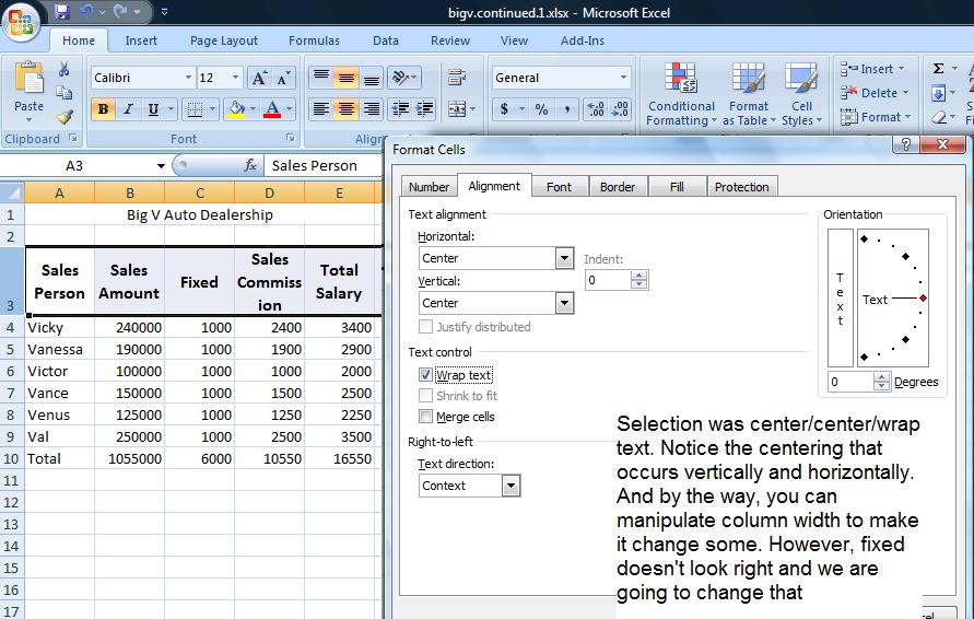
Click on format cells and you will se a dialog box pertaining to 6 possibilities for the range selected. One, protection, we will not deal with. Font generally can be dealt with using the font group of the home tab of the ribbon. Even number, which is very important, can be dealt with through the number group of the home tab. But alignment still holds importance and we want to click this. Notice there is a check box, merge cells, and in essence this was used to create the title in Row 1 although it is easier to control through the icon we used.
There are two combo boxes which control the type of formatting on a vertical and horizontal level. To start out, use center and center and click the wrap text check box. This is the most important of the control although you would not know it by the placement. Below we show a compoasite of these selections and the result.
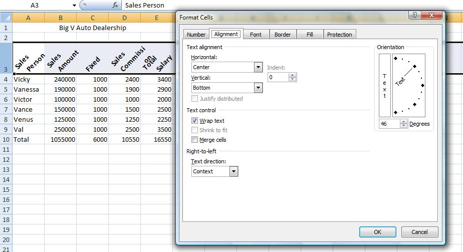
Fixed really should be at the bottom and this would have occurred if the vertical controls were set to bottom. Further, you might want to set this text at an angle and the picture below shows this using a 45 degree angle.
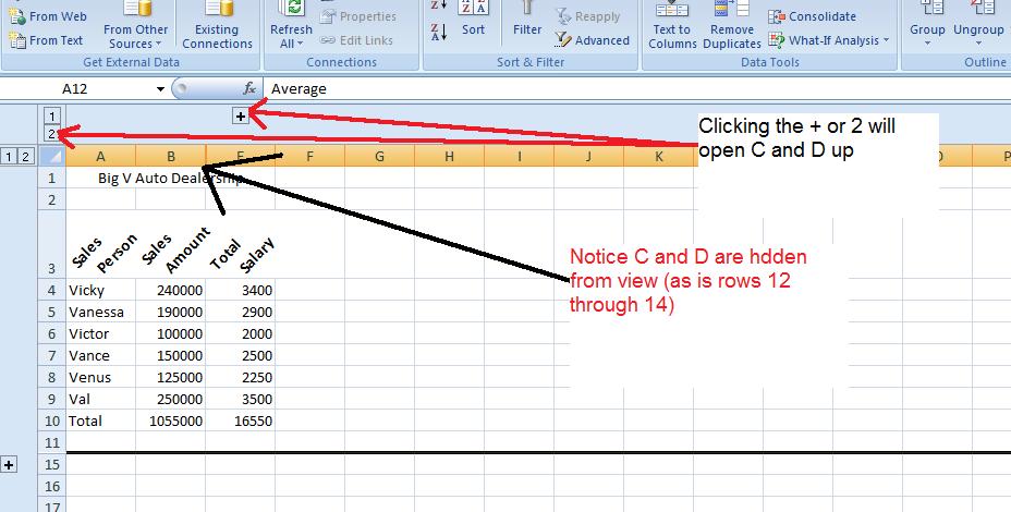
Now, having dealt with the titles, let's assume we want to prepare this for different viewers (different people in our organization). The needs of information are different for any of them. There is the owner who wants to know what amount was sold and what the salaries were. There is the accountant who need to see all numbers. To resolve this, Excel provides from grouping which on the operating system is called un Or decompress and compress. Here we have group and ungrouping of rows and columns. This is done on a specific entire row or column basis. Group and ungroup is found on the data tab of the ribbon.
Let's start this looking at columns C &D - fixed and variable. The big boss is probably not interested in this so highlight the entire column c and the entire column D by clicking insider the descriptor headings of c and D. Now, click group on the data menu. A new section opens up with new controls. Use of the controls (both to the left and above the columns) allows you to compress C & D from view or make them visibile. Similarly, let's do the same for rows 12, 13 & 14. hen compressed, by the way. a printout will not showe these columns and/or rows so this works even when printing. Below is an example of this.
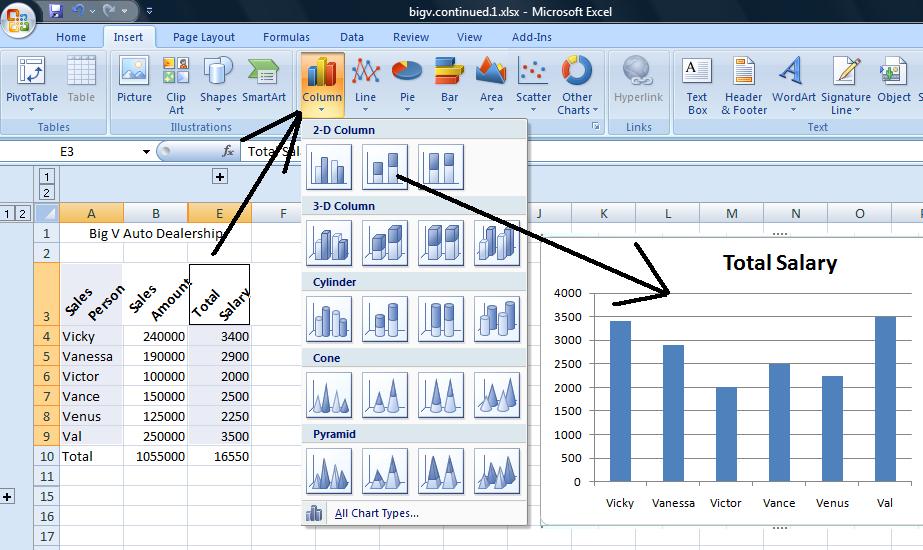
A graph or chart might look good here. Let's reference the sames person's name and show their salary. What type of chart would work to do this. Probably a bar/column chart. Microsoft calls that we woud normally call a Bar chart, a column chart. For this class bar abd column is interchangeable and you can do either when asked to do a bar chart.
Over the years, excel has made it easier and quicker to invoke a chart. Here's how easy it is. Drag you mouse over the names of the sales people including the column header, Sales person. Do not include total infor. You have selected a range, A3 through A9. Now, depressing your control key, extend the range by dragging your mouse over the salaries. Again include the column header by do not include the total. This is the extended range I alluded to previously and it is only with this type of charting that we will support it. Now, at the moment, A3 through and E3 through E9 have been selected and you should be able to see thiso nthe spreadsheet. Now, click the insert tab of tghe ribbon and hone in on the middle section of graphs. Click column and choose whichever "sub graph" you want to produce the chart. Below is a composite of this.
Finally, for today, let's format this spreadsheet somewhat. In previous versions there was a concept called autoformat that was invoked. In this version invoking format gives you a lot more than just formatting and we will look at that in the next problem we do. For this one, let's end up by setting the headers, blue and the totals red. Select the column headers. Right click and select format cells. Choose the fill tab and select a blue color. Similarly, select the totals. Right click and selec t format cells. Choose the fill tab and select a red color.
We can access where we left off on monday by clicking here.
We are at the point that we need to resolve each salesman;s salary.
We have one more column to calculate. The sum of fixed and variable. Let's sum up column C and D. E1 will be =c1+d1. Let's copy down. By E6, what do you think will be our formula. If you guessed =c6+d6, you are correct. And keep in mind, this is the same as =d6+c6.
While we are on the formula tab, let's indicate a new control for excel in this version and that is evaluate formula. It's use is better seen with more complicated formulas and you should use this as you study for your test in a few weeks, but it will show you the sequence of calculations that excel uses for get an answer for any cell. Move onto D6 and click this control and you will see these calculations in action.
While we are looking at calculation, this would be a good time to talk about ball parking. Excel does what you want it to do. There is no editorial comment from the program. It has no way of knowing or interpreting what is the ultimate purpose of these calculations. It is up to you to make sure that these calculations make sense. I use equivalents of 1% to determine if in the ballpark. !% is easy to deal with since you drop 2 zeros. In other problems 10% is the marker and yuo drop 1 zero. Let's assume that this problem was working with 1.2% commission. I'd still use 1% as my marker doubling the result to look at 2%. The end reult, when applying 1.2% should be between 1% and 2% and it should be biased closer to the 1%. Look at our calculation at this point 1000 for the monthly fixed should have looked somewhat correct based on the statement "12000 over the year". The number in the D column should correspond to 2 zeros being dropped from the values in B. Finally, the calculations should be easy enough to check the accuracy of column E.
Now, above, we did our summing for salary as the addition of two numbers. Is there another way. Yes! Contiguous cells can be designated as ranges and we can sum a range through the first of several functions we will study, Sum. The syntax of this is =sum(). c1 and d1 are the range c1:d1. Now, let's establish a new column, F, and put =sum(a1:b1) into the formula bar. Copy this down and if done right, you should get the same numbers as column E.
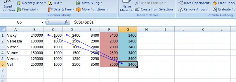
Let's continue. Sheet operations are independent unless you yourself change this. You have been working with sheet1 and probably have not realized that sheet2 also has calculation in it. Click on sheet2. Here's are problem again but with 2 columns. Look at the last column indicated in blue. We have been dealing with something called relational addressing. 3 other addressing schemes exist in Excel. For this class, we will deal with one other, absolute addressing. Using trace precdents, click on G6. You should see something like below which is very different than what we have seen before. This is crosiing rows. In absolute addressing, which is indicated by a $, you really are using the addresses indicated. Therefore $c$1 stays as $c$1 as a fill takes place.
Having dealt with absolute addressing, what about column F. The results look the same as E but the calculations are done very differently. We are using a function designated as =sum(). As with many functions, this can be widely used: as an example =sum(first, second, third, four) would be legitamate where first, second, third and fourth are something called ranges or cell or constants (in math). So, this brings up what is a range?
For this class (and this has changed with the additon of the use of the extended selection by way of the ctrl key) a mouse selection that resembles a rectanggle is a range. Take an example. Select c1. Drag your mouse through c6. C1 to c6 make a rectangle and a range. You can designate as c1:c6 or c6:c1. Similarly, we have the same situation with c1 and d1. They make the range c1:d1 (or d1:c1). By placing a range in the sum function, you can sum up all the elements (cells) indicated by the range. So, you see the f1 contains =sum(c1:d1). Ranges are similar to cell addressing in that they can be manipulated. One fill filled up column F.
Let's go back to our sheet1. Column totals wouldn't be a bad idea for B,C,D and E. Can you figure out the fastest way to do this. If you said range, you are correct. We'll show you two ways to do this as we are in class
Previously, we discussed relational vs absolute addressing (and we are using relational for this problem although I may show you an example of absolute at the end of this lecture, today. Manipulation of widths of columns and how Excel deals with numbers when the width is too small vs numerics. We looked at ranges and how these are used with the function Sum() and used Sum() (and autosum) in column totals among other things. You also saw how to turn the spreadsheet into a table of formulas. Now for today, we are going to deal with insertion of rows (possible columns) and setting up a set of column headers. Also, how to gruop columns (and rowsfvor the matter) and the creation of a very limited graph).
We are going to look at insertion. This can be done on many levels including insertion of a cell, a range, a row and a column. Unless you are at the row and column level, a second question is asked of you. Are you moving down the other cells by rows or by columns. You are not asked this question when a row or column is inserted. In additon, there are two ways of requesting insert. The one not recommended by me is the formal approach using the insert control on the home tab as indicated below.
In the case of an insertion of a row (or column) to use the context sensitive popup using the right click of the mouse. To do this, click the row that will move down when the new row is inserted. n the case of several rows being inserted at the same time, drag your mouse and select the number of rows where the first row will move down. In our example we need to add 3 rows. One for the title of the table, a blank and then the column header. Below, you see the start of this, Rows 1 to 3 are highlighted. A right click has made the pop up menu appear and we are about to click insert on that menu.
We can handle the title first and it can be as simple as the Big V Auto Dealership. We want this to center over our table. Insert Big V Auto Dealership in A1. It will bbleedc into b1 abd probably c1. Highlight the range a1:e1 and click the merge and center button in the alignment group of the home tab. What we've done here (as mentioned on Wednesday in class) is create a large A1 spanning to F1. And our result should look similar ot what we show below.
Now, we will allow the blank row to stay at row 2 as it is but now let's concentrate on the header row which we will put in row 3. Each cell of row 3 will provide header info for that column. But it's not going to look good as we first put it in. We will have to manipulate the row as you will see. But first, let's enter the info. Column A is Sales Person. Notice how it bleeds into the next cell. That next cell should be Sales Amount. Column C is fixed. Column D is sales Commission. And, finally, column E is total Salary.
One solution would be to widen the columns as demonstrated on Wednesday. While it will work, it will make the spreadsheet look odd with the columns being to big. WHat we would like to do is have the system break the cells so that there may be multi-leveled descriptions. And that's what we are going to do. But first, let's bolden these descriptions and increase the point size. With row 1 selected (and this is done by clicking in the descriptor of row 1 where it says 1), increase the point size to 12 and click the bold button.
Now, you have two choices as to selection. You can use the pop up menu as we have done before and select format cells or the format control on the home tab and select format vcells. Below we show both possibilities.
Click on format cells and you will se a dialog box pertaining to 6 possibilities for the range selected. One, protection, we will not deal with. Font generally can be dealt with using the font group of the home tab of the ribbon. Even number, which is very important, can be dealt with through the number group of the home tab. But alignment still holds importance and we want to click this. Notice there is a check box, merge cells, and in essence this was used to create the title in Row 1 although it is easier to control through the icon we used.
There are two combo boxes which control the type of formatting on a vertical and horizontal level. To start out, use center and center and click the wrap text check box. This is the most important of the control although you would not know it by the placement. Below we show a compoasite of these selections and the result.
Fixed really should be at the bottom and this would have occurred if the vertical controls were set to bottom. Further, you might want to set this text at an angle and the picture below shows this using a 45 degree angle.
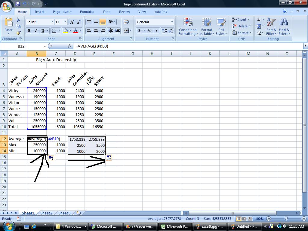
If you want, you can set this back. We now want to set up 3 rows below this table indicating for each column, max, min and average. Our table stretches to row 10 so let's use row 12 to start this. To get an averagbe, indicate a range in the =average() function. Likewise for max using =max() and min using =min(). So in B12, set the function =average(range) where range is B4 through B9. Why not use B10?
Similarly, in B13, set up the max and in B14, set up the min. Similar to our totals, these are relationships that can be copied over. But you do not have to do this a row at a time. Excel is smart enough to fill up ranges. Select the range B12 though B14 and then grab the handle and copy over. See how easy this is! Below is a composite of this.
We have our spreadsheet and then some. Suppose we would like to prepare it for a few viewers. But the needs are different for any of them. There is the owner who wants to know what amount was sold and what the salaries were. There is the accountant who need to see all numbers. To resolve this, Excel provides from grouping which on the operating system is called un Or decompress and compress. Here we have group and ungrouping of rows and columns. This is done on a specific entire row or column basis. Group and ungroup is found on the data tab of the ribbon.
Let's start this looking at columns C &D - fixed and variable. The big boss is probably not interested in this so highlight the entire column c and the entire column D by clicking insider the descriptor headings of c and D. Now, click group on the data menu. A new section opens up with new controls. Use of the controls (both to the left and above the columns) allows you to compress C & D from view or make them visibile. Similarly, let's do the same for rows 12, 13 & 14. hen compressed, by the way. a printout will not showe these columns and/or rows so this works even when printing. Below is an example of this.
A graph or chart might look good here. Let's reference the sames person's name and show their salary. What type of chart would work to do this. Probably a bar/column chart. Microsoft calls that we woud normally call a Bar chart, a column chart. For this class bar abd column is interchangeable and you can do either when asked to do a bar chart.
Over the years, excel has made it easier and quicker to invoke a chart. Here's how easy it is. Drag you mouse over the names of the sales people including the column header, Sales person. Do not include total info. You have selected a range, A3 through A9. Now, depressing your control key, extend the range by dragging your mouse over the salaries. Again include the column header by do not include the total. This is the extended range I alluded to previously and it is only with this type of charting that we will support it. Now, at the moment, A3 through and E3 through E9 have been selected and you should be able to see thiso nthe spreadsheet. Now, click the insert tab of the ribbon and hone in on the middle section of graphs. Click column and choose whichever "sub graph" you want to produce the chart. Below is a composite of this.
Unit 3 of your book does Excel under the title 'Electronic Spreadsheets.' For your own info, thec term derives from regular spreadsheets which are extended length ruled (as column and row) sheets of paper that bookkeepers and accountants have been using since the late 1800's.
We will be doing a different problem - one that emphasizes relative addressing. But, in following me, you should be reading and following the book although you will be using my test.
Excel is very mathematically oriented. It uses the mathematics you were taught between the 7th and 11th grade. If there was a question in your mind whether you would ever need that stuff, well, here it is.
Anyway, your instructor should have (or will) discuss the following points with you about excel as we start
For this week's class, let's do the handout - the Big w auto dealership which you can access below. This is a very rudimentary problem which is based on 1985 usage of excel. In dealing with this problem, we are starting our discussion of the nuts and bolts of excel. Starting from addressing we can deal with:
The hardest part of this is understanding relational addressing. Keep in mind that when you put =a2+1 into a cell, excel does not set this as the specific cell a2. if uses an offset (or difference) to tell itself how many rows and columns from the entered cell a2 is. If you are in a4 while putting in =a2+1, excel sets this as a offset of =2 rows, 0 columns. If you are in a1 and set =a2+1, the offset is 1 row, 0 column. If in c2, the offset to =a2+1 is 0 row, -2 columns and in the case of g5, the offset is -3 rows, -6 columns. It is this offset that is used for determining relationships. However, in the case of absolute addressing, =$a$2+1 for instance, a2 is always used.
If you understand relational vs absolute addressing, excel becomes very easy. A 2000 line item table (rows) is as simple as dealing with a 5 line item table with the only difference being the physical need to move through the line items. To this effect, Microsoft has developed the new construct, table, to deal with this. Now, in class, before dealing with the problem for the day, your instructor will show you some examples.
We are going to look at a problem that your instructor has previously done in classes. By time we're done, we will have done many of the techniques discussed in every Excel instructional book. But before we start, you must understand that the use of Excel has evolved over the years. The problems we are doing, and the techniques your book describes at the beginning are circa 1985 in use. Today, Excel is used as a supplement to database info (and similar type situations). There is an expectation that raw data is already available in some form (generally from a database although your instructor deals professionally with a set of problems where data is generally kept on excel spreadsheets) and that this information will need at minimum something called subtotaling. Once this is done, Excel's excellent chart (graph) tools finish up the project.
However, for our first problem, we are looking at entering our own data - we have no where to retrieve it from - and this data has already been subtotalled. Nevertheless, this problem should give us an idea about entering data and formulas, looking at the normal bias of excel, use of ranges and fills, use of various functions and the use of graphs.
So, if your instructor has not given you a handout - or you are going over what was done in class - let's bring up this problem and first discuss it in terms of what you know business to be and to need as far as information is concerned and then we'll start to apply some excel on it. Click here for the Big W auto dealership. Please note: I have changed the underlying document but the pictures (screen shots) use the previous instance of the BigV dealership.
Before discussing this problem, keep in mind that 6 salesmen is not a reasonable assumption today, In real life threr would have to be more salespeople and this is not even considering that most auto dealerships are chains. In doing this problem, we will handle it as if there were many more rows. This would be in preparation of further problems this term that will contain much more information.
In addition, all spreadsheets for commercial use have headers. We will ignore column headers as we start this problem and they will be put in later. Use A1 through A6 to enter the salesman's name. Use B1 through B6 to enter the amount sold for last month. Notice that excel is giving you informatiin as you enter the data. Non numeric data is left justified, Numeric data is right justified. Notice that Excel has not made any assumption on decimal points and as you put in an integer, that's what's there. Since this is money, should it be left as an integer? Do you have any other options when imputting? Yes, you could enter commas as separators but we will not be supporting that in this problem.
Even before putting anything else in, let's handle column width. Widths start out as standard. At minimun, you can manipulate column width by placing your cursor between two columns at the top (where the colunn indicators are) and use the cursor you aee at that point (I call it a grabber) to change column width. Below, you can see this in operation as both column widths have been decreased.
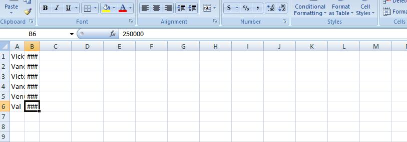
Besides the movement of the columns, look what happened to the data. Text is truncated. Numerics become first scientific notation (one of the allowable entries of numeric data on this system) and then pound signs. Excel is geared for math and it wants to make sure no decision is made on wrong assumptions. If it is trancated as done in string data, one might make a wrong decision seeing the wrong numeric entry. You can bring this back by invoking autofit for column width. A poll is taken on the width of each entry in a column and the widest entry determines the width of that column. If you can fit the widest, all the others will also fit, of course. There are ways to do this by the ribbon which your instructor will show you and by mouse. In terms of mouse, take the column in question and at the right gridline of the column description, double click.
In this problem, each salesperson gets $12000 a year split over the year. That is $1000 a month. Now, we could put in a 1000 for each entry next to a salesperson (column C), but we are going to use some math and relational operators to do the job. Math uses operators to determine what to do with numbers. Common operators (for real math and Excel) is + (addition) - (subtraction) * (for multiplication) and / (for division). To tell excel that you are dealing with a math operator, you need to start the entry with an equal sign (=). If you don't, you violate what excel feels is numbers and your entry defaults to text. The mathematics of this is 12000/12. Put this in at c1. Notice this is left justified and no calculation has taken place. Now try =12000/12. The equal sign indicates to exc el that we have a formula. 1000 shows up indicating that a calculation has occurred and it is right justified. Congradulations, you have done your first calculation albeit an easy one. Now, this is important. There are many things that make excel powerful and one is the ability to replacate relationships. The easiest relationship is a calculation. Move back into c1. There are 3 cursors in excel. The big plus sign is used to select cells and this is a way of creating ranges which we will talk about shortly. At the bottom right of any border in excel one would see a crosshair and put your cursor there now and you will see what I'm talking about. Finally, at the bottom left is both a crosshair and normal mouse cursor symbol combined. This is for moving and would be like a cut and paste in Word.
Now, in C1, move your cursor to the right bottom. When you see the crosshair, click your left button and drag the crosshair down the column. Below, you will see an example of this.
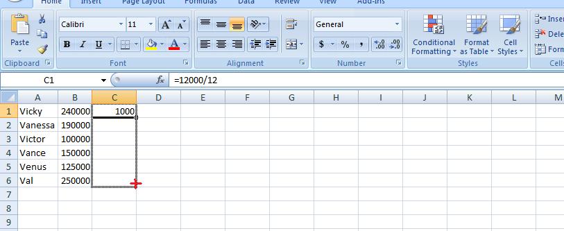
Let go of your mouse button and you will have copied this information. Waht was copied. Your relationship. You could see this by moving into each cell in column c and looking at the formula bar. It is easier to look at the screen with just formula. Go into the formula tab of the ribbon and on the right click show formulas. Below, you can see the result.
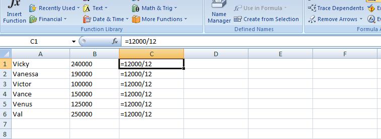
So you can see that you really did copy the cells as far as formulas are concerned. Now, hit show formula again to return to normal mode. We need to calculate the commission defined in our documentation as one percent of the sales amout for each salesperson. First, what is 1%. One could look at this as 1/100. Also as .01. And these are perfectly reasonable. But excel allows you to use 1% which is the easiest. Now, how do we calculate the first salesperson's commission (B1 for the sales, D1 for the result). We could use =1%*240000 or =240000*1% - this is one of the laws in our math which you should have learned in high school. This will work but it is limited. What would happen if the 240000 sales figure was changed (a late sale, a sale that was missed, or a busted sale where the figure goes down) WE would need to change this twice. One in B1 and the other, here, in D1. It is easier to reference the value of a cell than continually use the number. Therefore, our math relationship in D1 should be =1%*b1 or =b1*1%. Put this into your spreadsheet. Now, I am going to use E1 to put in what was originally proposed: use the math expression =1%*240000. Now, let's change B1 to 200000 (a sale of 40000 did not go through), Look at the result in your spreadsheet. Below, we have the example.
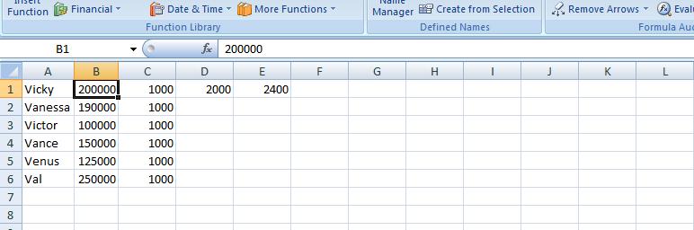
See the difference. The moral of this story: use references to cells. Now, let's do the same thing to column D that we did to C. Move your cursor to D1 and its right bottom border. Use the crosshair to fill down. Notice numbers are being put into the cells. They are 1% of what is 2 columns to the left. Use show formulas again and you will see what I have below
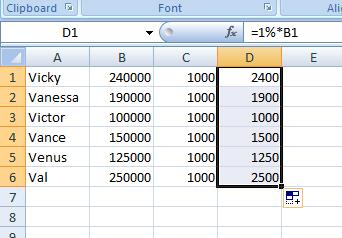
Notice that B1 was changed to B2 through B6 as we went along. You didn't do this. You had originally set B1. If B1 would have showed up, you would have been dealing with an absolute address. Excel determined that B1 was 2 columns to the left of D1 and 0 rows offset. As you filled into D2, the corresponding cell would be 2 columns to the left and 0 rows offset. Of course, we are therefore talking about B2 in this case and this was substituted. Look at the others: you will notice that this analysis is working for all these cells.
Now, look at D1. you should be able to see that it references b1. How does Excel look at this. Not as the cell b1. it looks at this as the cell 2 columns to the left. As we copy down this relationship, as it hits a cell and needs to enter a formula, the reference to a cell two columns to the left is enforced. Now copy this down to fill d2 through d6.
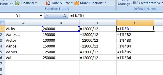 Previously, we have clicked within cells to see the formulas in the formula bar. Is there some way of doing this on a more geenral basis. Yes! In the formulas tab, on the right click show formulas and you will see what we have to the right. This is a good tool to use to see formulas in general as it lays it out on the spreadsheet. Ypu can even operate your spreadsheet this way in terms of entering formulas but you would not see the results. Your instrcutor would recoment that every now and then you click on this, especially if you have a big and complicated spreadsheet, to see if the patterns of the formulas make sense.
Click show formulas again and you are back to the regular aspect of excel. Excel has some other tools that you can use to get a feel whether you are proceeding as planned. Move your cursor to D1. Staying in the formula ribbon, click trace precedents and an arrow will appear emanating from B1. You can eliminate the arrow by using remove arrow/remove precedents. Precedent is a nice way of saying the di uses b1 in its calculation and b1 is 2 columns over to the left.
Reversely, click in cell b5 and click trace dependents. Notice the same type of arrow going from b5 to d5. On complicated spread sheets this can be a help to trace the flow of the data. Below, we have composited these two controls.
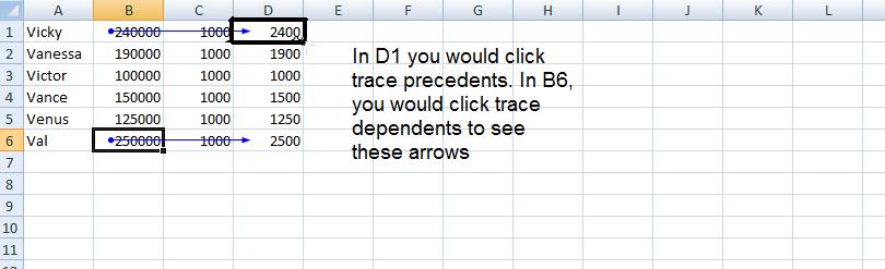
While we are on the formula tab, let's indicate a new control for excel in this version and that is evaluate formula. It's use is better seen with more complicated formulas and you should use this as you study for your test in a few weeks, but it will show you the sequence of calculations that excel uses for get an answer for any cell. Move onto D6 and click this control and you will see these calculations in action.
We have one more column to calculate. The sum of fixed and variable. Let's sum up column C and D. E1 will be =c1+d1. Let's copy down. By E6, what do you think will be our formula. If you guessed =c6+d6, you are correct. And keep in mind, this is the same as =d6+c6.
While we are looking at calculation, this would be a good time to talk about ball parking. Excel does what you want it to do. There is no editorial comment from the program. It has no way of knowing or interpreting what is the ultimate purpose of these calculations. It is up to you to make sure that these calculations make sense. I use equivalents of 1% to determine if in the ballpark. !% is easy to deal with since you drop 2 zeros. In other problems 10% is the marker and yuo drop 1 zero. Let's assume that this problem was working with 1.2% commission. I'd still use 1% as my marker doubling the result to look at 2%. The end reult, when applying 1.2% should be between 1% and 2% and it should be biased closer to the 1%. Look at our calculation at this point 1000 for the monthly fixed should have looked somewhat correct based on the statement "12000 over the year". The number in the D column should correspond to 2 zeros being dropped from the values in B. Finally, the calculations should be easy enough to check the accuracy of column E.
Let's continue. Sheet operations are independent unless you yourself change this. You have been working with sheet1 and probably have not realized that sheet2 also has calculation in it. Click on sheet2. Here's are problem again but with 2 columns. Look at the last column indicated in blue. We have been dealing with something called relational addressing. 3 other addressing schemes exist in Excel. For this class, we will deal with one other, absolute addressing. Using trace precdents, click on G6. You should see something like below which is very different than what we have seen before. This is crosiing rows. In absolute addressing, which is indicated by a $, you really are using the addresses indicated. Therefore $c$1 stays as $c$1 as a fill takes place.
Having dealt with absolute addressing, what about column F. The results look the same as E but the calculations are done very differently. We are using a function designated as =sum(). As with many functions, this can be widely used: as an example =sum(first, second, third, four) would be legitamate where first, second, third and fourth are something called ranges or cell or constants (in math). So, this brings up what is a range?
For this class (and this has changed with the additon of the use of the extended selection by way of the ctrl key) a mouse selection that resembles a rectanggle is a range. Take an example. Select c1. Drag your mouse through c6. C1 to c6 make a rectangle and a range. You can designate as c1:c6 or c6:c1. Similarly, we have the same situation with c1 and d1. They make the range c1:d1 (or d1:c1). By placing a range in the sum function, you can sum up all the elements (cells) indicated by the range. So, you see the f1 contains =sum(c1:d1). Ranges are similar to cell addressing in that they can be manipulated. One fill filled up column F.
Let's go back to our sheet1. Column totals wouldn't be a bad idea for B,C,D and E. Can you figure out the fastest way to do this. If you said range, you are correct. We'll show you two ways to do this as we are in class
Previously, we discussed relational vs absolute addressing (and we are using relational for this problem although I may show you an example of absolute at the end of this lecture, today. Manipulation of widths of columns and how Excel deals with numbers when the width is too small vs numerics. We looked at ranges and how these are used with the function Sum() and used Sum() (and autosum) in column totals among other things. You also saw how to turn the spreadsheet into a table of formulas. Now for today, we are going to deal with insertion of rows (possible columns) and setting up a set of column headers. Also, how to gruop columns (and rowsfvor the matter) and the creation of a very limited graph).
We are going to look at insertion. This can be done on many levels including insertion of a cell, a range, a row and a column. Unless you are at the row and column level, a second question is asked of you. Are you moving down the other cells by rows or by columns. You are not asked this question when a row or column is inserted. In additon, there are two ways of requesting insert. The one not recommended by me is the formal approach using the insert control on the home tab as indicated below.
In the case of an insertion of a row (or column) to use the context sensitive popup using the right click of the mouse. To sdo this, click the row that will move down when the new row is inserted. n the case of several rows being inserted at the same time, drag your mouse and select the number of rows where the first row will move down. In our example we need to add 3 rows. One for the title of the table, a blank and then the column header. Below, you see the start of this, Rows 1 to 3 are highlighted. A right click has made the pop up menu appear and we are about to click insert on that menu.
We can handle the title first and it can be as simple as the Big V Auto Dealership. We want this to center over our table. Insert Big V Auto Dealership in A1. It will bbleedc into b1 abd probably c1. Highlight the range a1:e1 and click the merge and center button in the alignment group of the home tab. What we've done here (as mentioned on Wednesday in class) is create a large A1 spanning to F1. And our result should look similar ot what we show below.
Now, we will allow the blank row to stay at row 2 as it is but now let's concentrate on the header row which we will put in row 3. Each cell of row 3 will provide header info for that column. But it's not going to look good as we first put it in. We will have to manipulate the row as you will see. But first, let's enter the info. Column A is Sales Person. Notice how it bleeds into the next cell. That next cell should be Sales Amount. Column C is fixed. Column D is sales Commission. And, finally, column E is total Salary.
One solution would be to widen the columns as demonstrated on Wednesday. While it will work, it will make the spreadsheet look odd with the columns being to big. WHat we would like to do is have the system break the cells so that there may be multi-leveled descriptions. And that's what we are going to do. But first, let's bolden these descriptions and increase the point size. With row 1 selected (and this is done by clicking in the descriptor of row 1 where it says 1), increase the point size to 12 and click the bold button.
Now, you have two choices as to selection. You can use the pop up menu as we have done before and select format cells or the format control on the home tab and select format vcells. Below we show both possibilities.
Click on format cells and you will se a dialog box pertaining to 6 possibilities for the range selected. One, protection, we will not deal with. Font generally can be dealt with using the font group of the home tab of the ribbon. Even number, which is very important, can be dealt with through the number group of the home tab. But alignment still holds importance and we want to click this. Notice there is a check box, merge cells, and in essence this was used to create the title in Row 1 although it is easier to control through the icon we used.
There are two combo boxes which control the type of formatting on a vertical and horizontal level. To start out, use center and center and click the wrap text check box. This is the most important of the control although you would not know it by the placement. Below we show a compoasite of these selections and the result.
Fixed really should be at the bottom and this would have occurred if the vertical controls were set to bottom. Further, you might want to set this text at an angle and the picture below shows this using a 45 degree angle.
If you want, you can set this back. We now want to set up 3 rows below this table indicating for each column, max, min and average. Our table stretches to row 10 so let's use row 12 to start this. To get an averagbe, indicate a range in the =average() function. Likewise for max using =max() and min using =min(). So in B12, set the function =average(range) where range is B4 through B9. Why not use B10?
Similarly, in B13, set up the max and in B14, set up the min. Similar to our totals, these are relationships that can be copied over. But you do not have to do this a row at a time. Excel is smart enough to fill up ranges. Select the range B12 though B14 and then grab the handle and copy over. See how easy this is! Below is a composite of this.
We have our spreadsheet and then some. Suppose we would like to prepare it for a few viewers. But the needs are different for any of them. There is the owner who wants to know what amount was sold and what the salaries were. There is the accountant who need to see all numbers. To resolve this, Excel provides from grouping which on the operating system is called un Or decompress and compress. Here we have group and ungrouping of rows and columns. This is done on a specific entire row or column basis. Group and ungroup is found on the data tab of the ribbon.
Let's start this looking at columns C &D - fixed and variable. The big boss is probably not interested in this so highlight the entire column c and the entire column D by clicking insider the descriptor headings of c and D. Now, click group on the data menu. A new section opens up with new controls. Use of the controls (both to the left and above the columns) allows you to compress C & D from view or make them visibile. Similarly, let's do the same for rows 12, 13 & 14. hen compressed, by the way. a printout will not showe these columns and/or rows so this works even when printing. Below is an example of this.
A graph or chart might look good here. Let's reference the sames person's name and show their salary. What type of chart would work to do this. Probably a bar/column chart. Microsoft calls that we woud normally call a Bar chart, a column chart. For this class bar abd column is interchangeable and you can do either when asked to do a bar chart.
Over the years, excel has made it easier and quicker to invoke a chart. Here's how easy it is. Drag you mouse over the names of the sales people including the column header, Sales person. Do not include total info. You have selected a range, A3 through A9. Now, depressing your control key, extend the range by dragging your mouse over the salaries. Again include the column header by do not include the total. This is the extended range I alluded to previously and it is only with this type of charting that we will support it. Now, at the moment, A3 through and E3 through E9 have been selected and you should be able to see thiso nthe spreadsheet. Now, click the insert tab of the ribbon and hone in on the middle section of graphs. Click column and choose whichever "sub graph" you want to produce the chart. Below is a composite of this.
Today is our last lecture on Access. In fact, we will use a query to create an excel spreadsheet. It is expected that the rest of the week will involve the librarian lecture so the next lecture on Excel will be next Mon, Nov 14th.
In terms of access, we are going to do several other "joins" and then look at aggregate functions. You can access the database by clicking here.
I have put a query into the database called pop per sqmi. One class got to this, the other did not. so let's start with a join. Add to the tables being shown with capitals. if not already, set the link between state of states and state of capitals as shown below.
Here's the power of relational databases. Links designated as joins allow the interchange of information between tables. inner joins, the one we have here, go 1 to 1. If somethng is missing in either table, it is not shown in the result. Left joins in Access (and Access does not do all the possible combinations that higher level SQl databases allow) look at states, and state within states. All the entries of states.state are shown even if a link does not exist. The same on the other side, known as a Right join. All of Capitals.state would be shown whether or not a corresponding link is available in States.state. Below, we see the beginning of this.
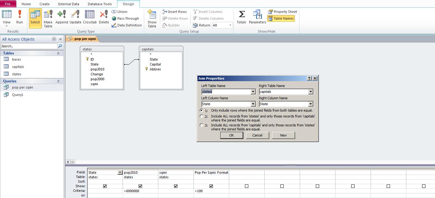
The easiest way to add a column in the grid is to highlight where it should show and click insert columns above in the design tab. Below, we've done that.
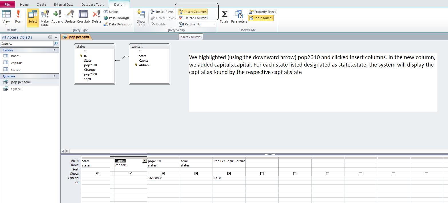
Let's finish this out by adding the bases table similar to what we did for capitals. Notice the bases table has abreviations for state designations. Abbreviations also exist in capitals. If it doesn't do it already, set a link from abbrev in capitals to abbr in bases. This should prove to you that there is no need for field (or column) names to be consistent between tables. Now, let's add as fields base and employees from bases and run that. The result should be similar to what's below.

Notice that we have shattered our 1 to 1 relationships. There are many bases per state in most cases and thios is what is shown. Because Access is a lower level SQl database, it is not as flexible as other SQL databases and you will have limitations as to inner, right and left joins. Generally I have found that Access will access a SQL statement consisting of all inner joins, all right joins or all left joins. We mention this because there are bases in all the states and we are only displaying those bases in states with pop2010 > 6 mil and pop density > 100.
We would like to determine the population of the 50 states. To do this, we invoke aggregate functions. Here's where there are real limitations to how SQL is syntaxed. Let's start slowily. In SQL view, just put in select sum(pop2010) from states. The result is 309183463. The sum is an aggregate function. Let's find out the state average. Substitute avg for sum. The average state has 6183669.25 population. All right. Go into design view. You can see a total row has been added which allows you to enter these aggregate functions. Now, add the bases table. We would in addition like to find out all the employees of the bases per state. Notice, we have no link. States are spelled out in states, abbreviated in bases. Let's add the capitals table to rectify this. If the links don't show up, set them.
Now, let's add state name as the first column. Somethng been added. Do you see the group by. Without group by, SQl stops in its tracks. Aggregate cannot be displayed with specific line item info in Sql unless that line item data is acknoledges to be a group by. QBE handles this for you; Sql view does not. To finish this problem, click for employees. The system with set group by as a default. Click for sum. ANd then let's run. If you did this right, you have the population for the atate and the sum of the employees for the bases that reside in the states. Below, we show this,
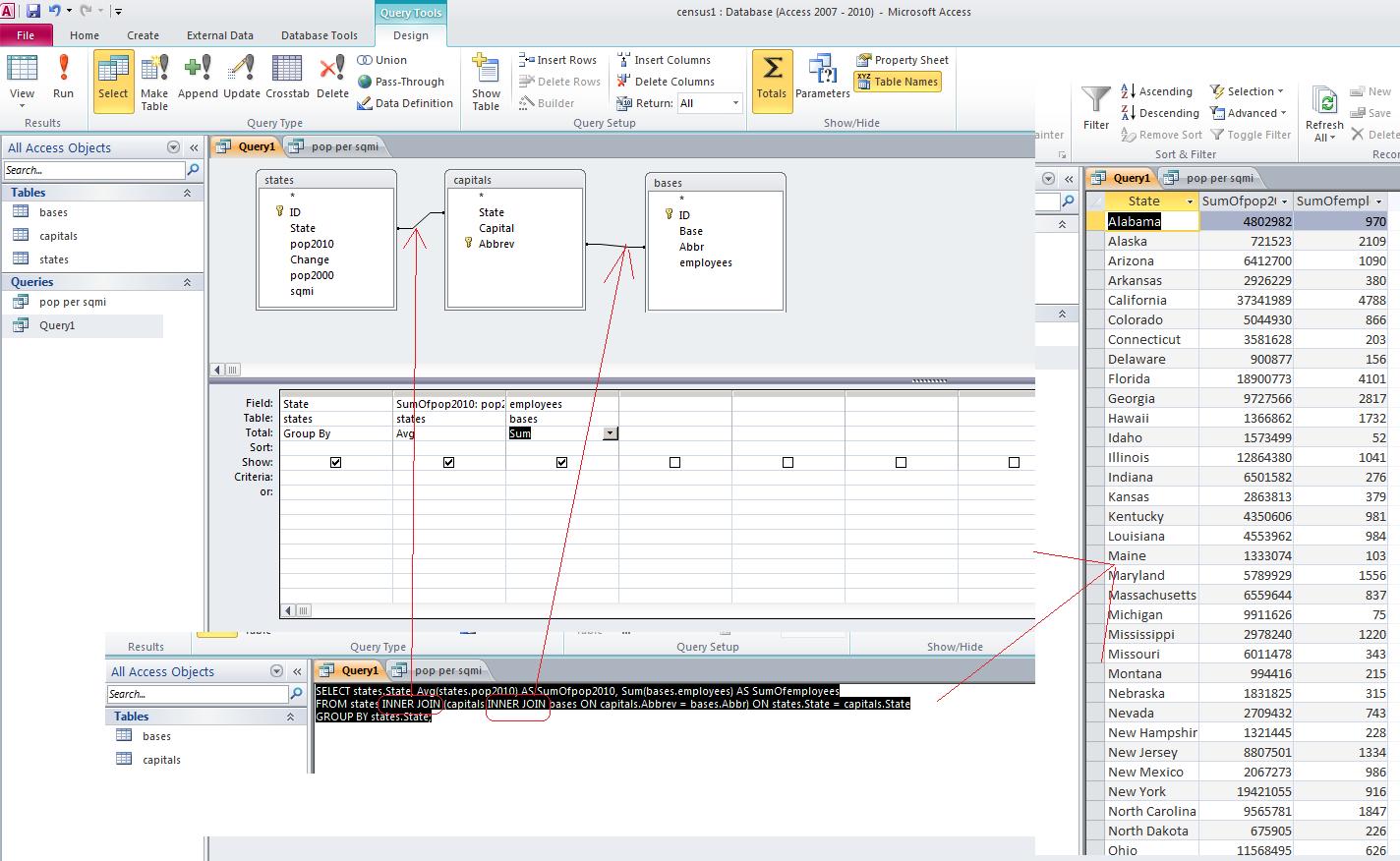
Let's export this into an excel spreadsheet. Save this query by clicking the x on the right top side. Now, where Query1 shows on the right (you may have a different name) right click and choose export. Just like with import, there are plenty of options but we are interested in excel. We are now going the other way. Notice that the name defaults to query1.xlsx and you can rename this. There is no need to keep the formatting. Using the continue or OK, we have created an excel spreadsheet. For the reaminder of the class we will talk about Excel. Number of row, number of columns, number of sheets. Question of width of columns and how to set. And, we will try to do some aumations and averaging.
I have made some changes to the census database. In the states table, I have added the fiekd sqmi, which represents the square miles of the individual states. You can access this database by clicking here.
Now, let's start where we left off on Monday, but this time adding in the filed sqmi. Let's show those states with populations of 6 million or more. Into the create tab, query design. Indicate the states table. Set fields to show of state, pop2010 and sqmi. Set a criteria of >600000 for pop2010 as well as a descending sort as shown below. Also shown below, under the QBE commands, is the result.

Remember, QBE is another representation of SQL. Clicking on SQL view will display the SQL statement. The only addition will be states.sqmi to the select list for display. In the SQL window, let's try to do a calculation. What if you wanted to know the population per sq mi for each state. mathematically this is pop201/sqmi. Let's add this to the SQL statement. Your statement should now read as indicated below (and below that is the result)
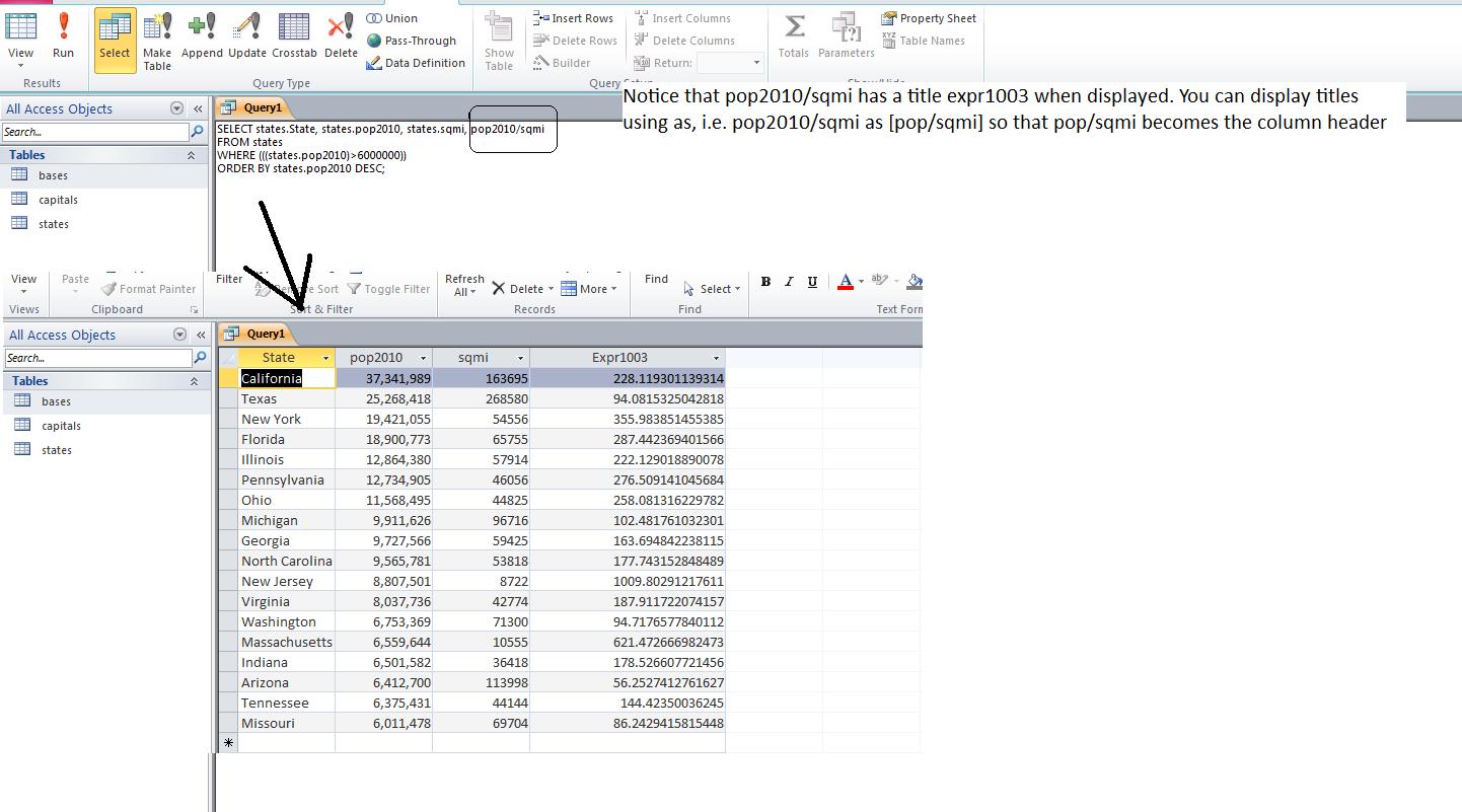
As an aside, and something you are not going to be responsible for, California's 228.1193011 has a bit too many decimal points. SQL has a function designated as format which you can use to resolve this. Suppose you wanted to make this into 2 decimals, a format string of ####.## - where # represents a plceholder for a number - would do, although #.## will also work. Your SQL statement might include format(pop2010.sqmi,"####.##") AS [POP/SQMI]. One other thing that you are already seeing. We already mentioned in class that formally columns (fields) should be designated by their table. So, we should have really used states.pop2010/states.sqmi. In additon, there is no requirement that embedded blanks not be used in a field name. For our class, I have tried not to put such blanks in. But, if I have used sq mi instead of sqmi, I would have been required to indicate this field name within brackets so we would have seen pop2010/[sq mi].
Now, we want to move along. What if we wanted to see those states with populations of 6 million who have pop/sqmi of 100 or greater. Let's do this through QBE. We get to that through the design view option of view. Notice how QBE is handling our sql statement. A new column has been added and you should see something like pop/sqmi:[pop2010]/[sqmi] or pop/sqmi:format([pop2010]/[sqmi],"#.##") if you have added formatting to 2 decimal point capability. In this column, let's set up a criteria for >= 100 which you should put into the criteria cell for this calculated field. Below, we've done this. The results have changed. Several states, including Texas and MIssouri are missing as they didn't meet the 100 standard. I've also indicated the SQL statement equivalemt. Notice the AND that has been added which we are about to discuss.
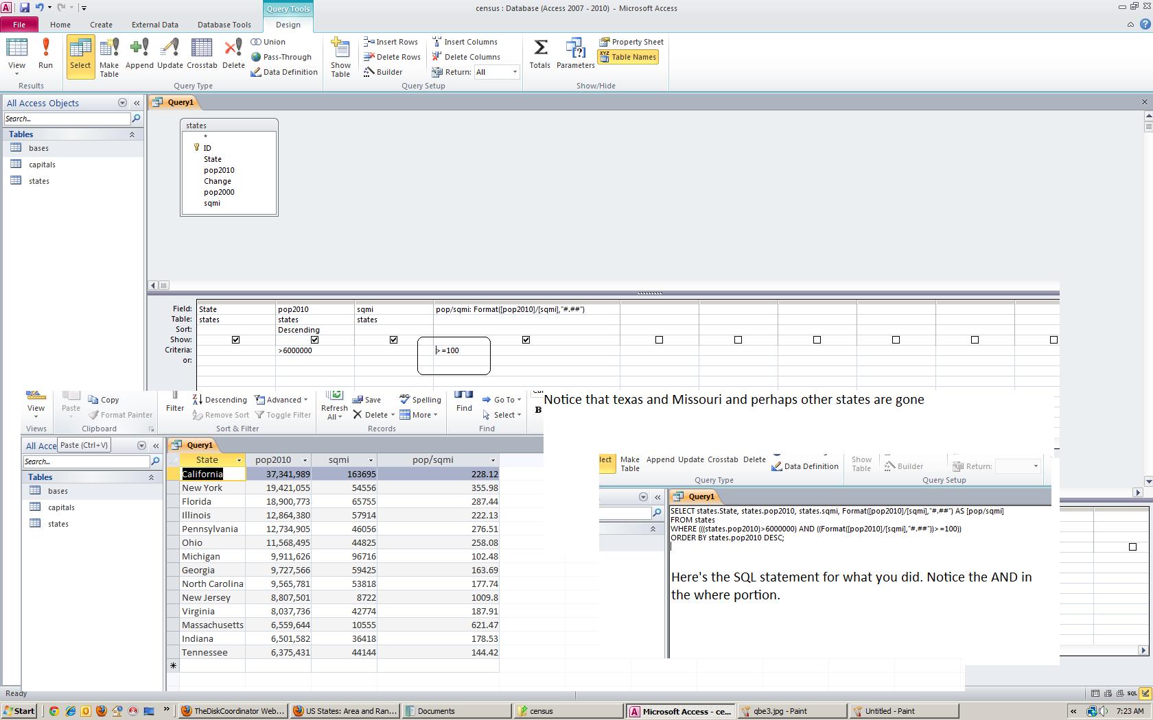
AND (also designated as logical and) is a boolean operator. Other operators are OR (or logical or), not and exclusive or. These become the basis of logical operations for databases and you see one here. When the librarian comes in, (s)he will show you examples of this. Below, I show this as a venn diagram.
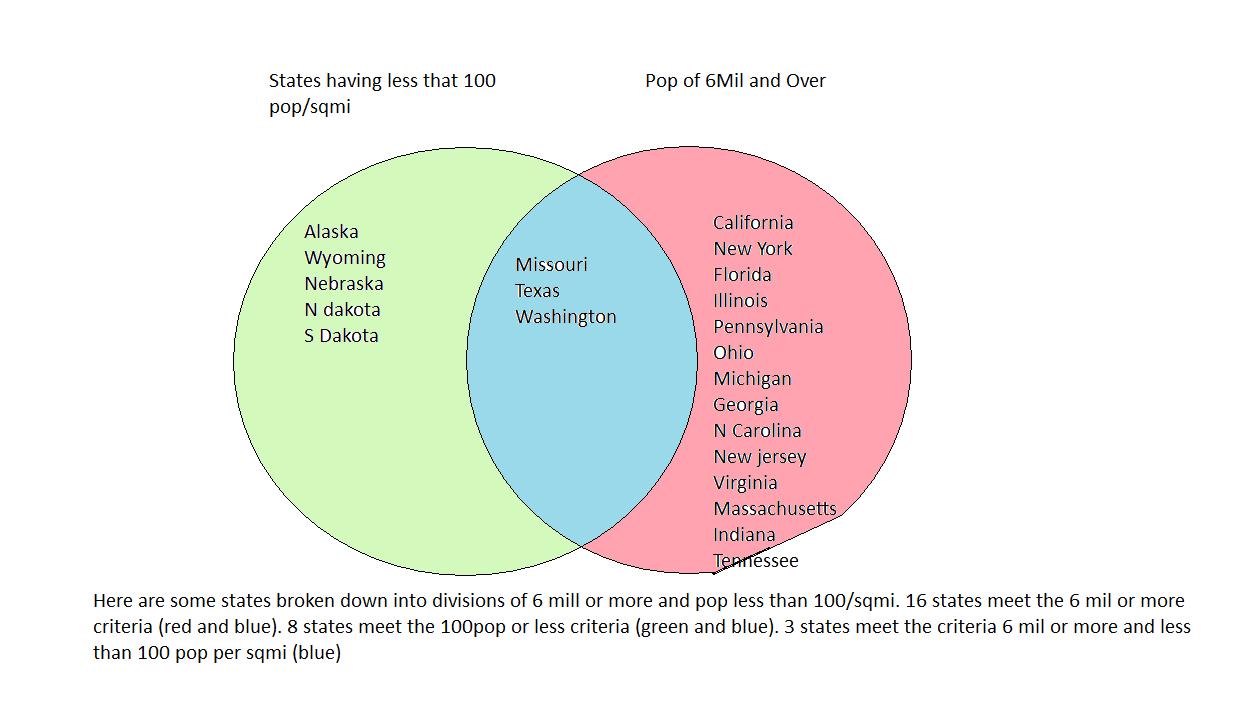
logical operators work on events. With two events, a determination of true or false is derived by whether the event is true or falsee. Assume that States having less than 100 pop/sqmi is designated as A and States haveing pop < 6 mil is B. A And B is designated by the color blue. A or B is designated by all three colors. On the board we'll give you a little more info on this. It is important in database operations to understand boolean operators. You can get through Excel without tihs knowledge although even in Excel this can facilitate calculations.
Now, with this, let's do a logical and and logical or problem. Determine the states that have population between 4 million and 10 million. It is easier to do this through SQL than QBE. Click on SQL view and locate the where. Delete from where to order and substitute pop2010>4000000 and pop2010<10000000. Running this we reveal the states Kentucky to Michigan. Now, look at QBE and you can see how this AND has been handled in this case. You could have done this differently. In the first instance of pop2010, set a criteria of >4000000 and set a second instance of pop2010 to <10000000. Below, we show both situations.

How do you tie in two or more tables. This is the forte of relational databases. in our example, what if we wanted to add the capital to the printout. In Qbe, right click the top and request show table, Click capitals as that is the table with tihs info. Either a link will be shown or we have to establish it. Links generally go to similar info. Generally, also, these columns that are linked are primary keys although that;s not required. Our link here should be from states.state to capitals.state. Once you have this, add a column below. Notice the fields indicate both tables, so select capitals.capital. Below we show QBe and the result.

Sql handles combination of tables by the use of joins. There is inner join and used here and outer join which brreaks down into a left join and right join. The join operation asks the program to match up the instances of the data in the columns designed as relational. You can see that Michigan has Lansing as its capital. When Access saw Michigan in the states table, it searched for Michigan in the capitals table and supplied that entry of Lansing to the result. You can get a feel for what the system is trying to do by returning to QBE and right clicking the pointer between the tables. Select properties and you will see a dialog box which gives you all the possibilities of the joins. We have the first radio button selected. If an entry doesn't exist in the reciprocal table, it is not included in the list that's produced. You can see the Left and Right join possibilities as indicated in radio button 2 and 3.
Last time in class we began to create an access database. We had created a table pertaining to the US census. Each entry of the table pertained to the census for each state - population in 2010, population in 2000 and the change between both.
I finished that table rfor us and extended it. This database now has tate capitals and abbreviations in another table and a third table contains US Military bases and the state (abbreviated) where they exist.
You can pull us this database by clicking here. When we were looking at the one table, it was possible to enter info one row and column at a time. But, in real life, you try to create the data at another location and then import it in. Click here for an excel spreadsheet that contains the census data.
Like anything else in access, you cannot have two tables of the same name. So, we will create a state1 table (which will be exactly the same as the state table) by importing the uspop excel file into the census data base. Over many years, Access has developed a large repertoire of code for importing data.
One thing we should define. There is a difference between a linked and imported file. A linked file continues to remain independent of the Access structure. It can be deleted which will destroy your link. An imported file will physically exist with Access. While the original data is outside of the database, the original data is not used in Access calculations or procedures. Below, we show some composites as uspop.xlsx is brought into access as a table. We need to name it something other than state as state is already taken.
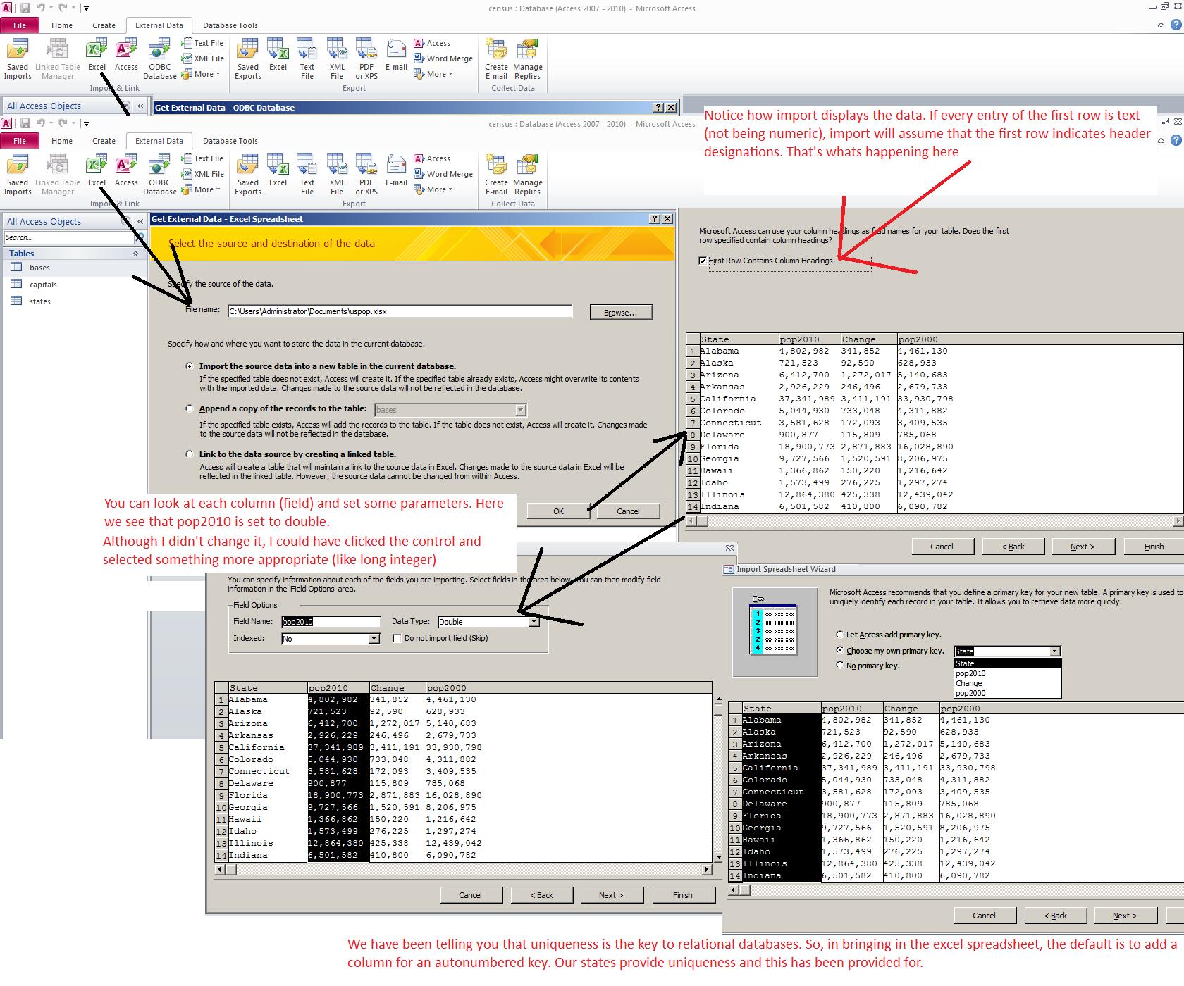
While we are not going to use it, Access allows the user to assign relationships to the tables. Here is where the term 'relationa;' has its meaning. Even though the names of the columns are different, abbr of bases relates to abbrev of capitals. In a like manner state of states relates to staste of capital. It is through these relationships that the power of relational databases is displayed because through this you can interrelate various information from different tables for one 'entity'. Below, we see these relationships

Now, the rest of the lecture pertains to SQl and QBE. We can use one to show the other although SQL goes through statements. Statements start with action items such as select, delete, update, insert, etc. We are going to be concentrating on the select statement. The full syntax for the select statement is select ? from ? where ? order by ? group by? having ?. For today, we are at select ? from ? where ? order by ?
Click create and then query design. Below, you will see the the result. You are in QBE (query by example). You must select a table and that should be states. Once selected you will see the states table above and it willl display all the columns in the table. We are starting very slowly. Let's assume we want to list all the states that have a population of 6 million or more. We would like to see the state name and population, We might as see these in reverse order with the most populous state shown first. Below, in the gride, click the control on the first instance of field. If you take states*, it will show every column as * is a default for all columns. Pick state. Show should now be checked. Move to column 2. Same thing but this time click pop2010. Show should be set. Click the sort row and pick descending. Above, a new tab is available designated as query design. Click the run (exclamation point) symbol. We have not chosen a population to stop at so you will see all the states displayed in descending pop order. Click view but this time look at sql view. You should see select states.state,states.pop2010 from states order by states.pop2010 desc. Now, let's impose the 6 million pop limit. Before order by, type in where pop2010>6000000. With only one table being selected, the system will recognize that we are dealing with the states table. Your sql statement should look like select state, pop2010 from states where pop2010>6000000 order by pop2010 desc. Click the run command. Now, you should have a response where all the states are above 6 mill in pop. Nolw, this time, click view design view. Notice that an additional column has been created. Is there a need for this. No. You could have set the constraint of >6000000 in the first pop2010.

These type of databases allow the user to ask questions. What states had 6 mill pop in 2000. Has any been added. In QBE, goto the next column. Indicate pop2000 as the column (field) and set the criteria of >6000000. Run this. Notice that we stop at indiana. Now, take a look at SQL. A little bit more complicated. We are into the world of boolean operators and "and" is one of them. We discuss this more in class.
Well, we hope to be back for these lectures. This has not been the easiest of procedures but this is sometimes how life is.
For the next two weeks, we hope to deal with Unit 4, Library and databases. One of the lectures during this period should be the librarian's lecture on peer reviewed sources of information.
Today, we do a little history on databases. You may remember the start of this semester when we discussed Harry Holerith and his sorting and collating machines. What was he attempting to resolve. It was a request for proposal from the US Government to resolve the US census for 1880.
The census of this country - determining the population of each state and the makeup of that population - is in actuality a database. So, in reality, what we call computer science and possibly data processing, begins with the need to manage databases (in addition to the need for fast calculation).
Below, is the latest census (supposedly) for this country
State 	        Population in 2010	Change through the decade	Population in 2000
Alabama	        4,802,982	        341,852	                    4,461,130
Alaska	        721,523	            92,590	                    628,933
Arizona	        6,412,700	        1,272,017	                5,140,683
Arkansas	    2,926,229	        246,496	                    2,679,733
California	    37,341,989	        3,411,191	                33,930,798
Colorado	    5,044,930	        733,048	                    4,311,882
Connecticut	    3,581,628	        172,093	                    3,409,535
Delaware	    900,877	            115,809	                    785,068
Florida	        18,900,773	        2,871,883	                16,028,890
Georgia	        9,727,566	        1,520,591	                8,206,975
Hawaii	        1,366,862	        150,220	                    1,216,642
Idaho	        1,573,499	        276,225	                    1,297,274
Illinois	    12,864,380	        425,338	                    12,439,042
Indiana	        6,501,582	        410,800	                    6,090,782
Iowa	        3,053,787	        121,864	                    2,931,923
Kansas	        2,863,813	        169,989	                    2,693,824
Kentucky	    4,350,606	        301,175	                    4,049,431
Louisiana	    4,553,962	        73,691	                    4,480,271
Maine	        1,333,074	        55,343	                    1,277,731
Maryland	    5,789,929	        482,043	                    5,307,886
Massachusetts	6,559,644	        204,076	                    6,355,568
Michigan	    9,911,626	        -44,203	                    9,955,829
Minnesota	    5,314,879	        389,209	                    4,925,670
Mississippi	    2,978,240	        125,313	                    2,852,927
Missouri	    6,011,478	        405,218	                    5,606,260
Montana	        994,416	            89,100	                    905,316
Nebraska	    1,831,825	        116,456	                    1,715,369
Nevada	        2,709,432	        707,400	                    2,002,032
New Hampshire	1,321,445	        83,030	                    1,238,415
New Jersey	    8,807,501	        383,147	                    8,424,354
New Mexico	    2,067,273	        243,452	                    1,823,821
New York	    19,421,055	        416,082	                    19,004,973
North Carolina	9,565,781	        1,498,108	                8,067,673
North Dakota	675,905	            32,149	                    643,756
Ohio	        11,568,495	        193,955	                    11,374,540
Oklahoma	    3,764,882	        306,063	                    3,458,819
Oregon	        3,848,606	        420,063	                    3,428,543
Pennsylvania	12,734,905	        434,235	                    12,300,670
Rhode Island	1,055,247	        5,585	                    1,049,662
South Carolina	4,645,975	        620,914	                    4,025,061
South Dakota	819,761	            62,887	                    756,874
Tennessee	    6,375,431	        675,394	                    5,700,037
Texas	        25,268,418	        4,364,424	                20,903,994
Utah	        2,770,765	        534,051	                    2,236,714
Vermont	        630,337	            20,447	                    609,890
Virginia	    8,037,736	        937,034	                    7,100,702
Washington	    6,753,369	        844,685	                    5,908,684
West Virginia	1,859,815	        46,738	                    1,813,077
Wisconsin	    5,698,230	        327,020	                    5,371,210
Wyoming	        568,300	            72,996	                    495,304
Looking at this data, which is not formatted correctly, what would you want to know and how would you describe this to a third party.
First, you probably would tell this third party that they are looking at a table of 2010 census data. This table is one of 23 tables indicating US population from 1790 to the present for every 10 years. In today's parlance, these tables would make up a database.
Each of these tables are composed of elements and the use of the words to describe these elements depends on your experience with database theory over the years. If you had grown up dealing with databases prior to 1980, you would say that the table above is composed of 50 records (each record representing a state) and each record has 4 fields (name, 2010 pop, change over the decade and 2000 pop).
By 1980, the theory of databases had changed and you would now be looking at 50 rows with each row representing a state. Each row would consist of 4 columns and you can guess what they would be. In addition, this table wouldn't do much if the state names and the numbers were intermixed and this brings up the term type and typing.
Columns (or fields) must be consistent as far as data is concerned. Specific typing is required. At the least, columns must be designated as alpha or numeric. Numeric can break down very easily into small and large integer, single and double floating point (for those familiar with Excel, Excel does mathematics in doule precision floating point) and logical. In many cases, this typing is consistent with the computer's architecture.
We can understand that you probably are very ho-hum pertaining to the differences between pre 1980 and post 1980 (although the break occurred in 1971 officially). But, this is more than just a nominal change in definition. 1971 marks the point where databases become uniform and consistent, but more on that later.
Let's continue to look at this data above. With its availability, what info would you want to know that it can give you beyond the specific numbered data you see above.
First, if you are not familiar with this country, you might want to know how many states are there. This can be resolved by counting the records and is known as a count. Perhaps, you would like to know how many states have a population of 6 million or above and this is count with a filter, the filter being the test that the state population be over 6 million. Filter is probably the proper term for this but in reality other terminology is used to describe this. SOme people would say qualifiers, some would say constraints, but you get the idea.
Another thing you might want to discern from this table is the entire population of the United States since it would consist of summing these 50 states (although in reality several territories and dependencies are not covered including the district of columbia). This is called a sum (some call it a total) and sums work only on mathematical columns. Again, filtering would be allowed just in case you want to find out the population of the US where residents live in states with population greater than 6 million.
You might want to determine the average population of a state. This, mathematically, is the total population divided 50, the number of states. This is known as an average and you would want this system to be able to handle this.
At the moment what has been explained is a flat file database. However, remember that we had another 21 or 22 tables with information. If we could "relate" this table to the other tables, we have moved this database and its tables to a higher plateau. We might be in the realm of what is called relational databases.
As computers become available in 1948, the first several years of databases are flat file situations dependent on the architecture of the machine and the facilitiy for holding the data. Originally, cards were used starting with one card per record. Later, multiple cards per record were programmed. Cards would allow only for text entry and numbers could be put in but only digit by digit needing to be modified once in the machine to numeric types allowable for mathematics.
In the early 1950's multiple attempts are tried to move off of cards. Magnetic tapes are used and mag tape holds card images but reference these mush faster. But, al imitation prevails. Cards and Mag tape are sequential. You cannot access a specific record without going through all the records the exist before it. This still puts a crimp on database usage. Consider for yourself the following: A 1950 or so help desk for master card where you call about your particular account. To access your account, the operator would have to wait for the computer to access all the accounts before yours before (s)he could start to work on you.
Attempts are made to expand the media. One attempt that was unsuccessful should be noted here. Univac attempts to put data into a radio orbit, using radio waves to move around the stratoshere holding relevant data. They can get it to move around the earth and retrieve it, but, not surpringly, the same problem with mag tape and cards exists: how do you retrieve it when you specifically need it.
In the end, something round and circular willould do and the creation of two possible pieces of equipment were considered. One was designated as a data set, the other a hard disk drive. A dataset was a cut up circle. Each arc (what the cut up would create) was made up of multiple surfaces which could be read. If you don;t cut up the circle, you have several planes that, with the appropriate readers while whirling at high speed, also can access data. Notice that this type of machinery gives the possibility of accessing records directly and this brought up the major change in databases of the late 50's, early 60's: Sequencial, indexed sequencial and direct. And this is what you would be studying if dealig with databases in that era.
Most companies hired programmers to specifically create their database. Any support ran through the manufacturer of the computer that this database was on. Except for the question of record and field and typing of the field, everything was specificaly done per site. Accessing of the database was done several times a week to create reports. There was no virtual, real time accessing capability due to the lack of equipment to do this.
Some database vendors were created during this time. A addon program would be a program that could take the data and sort it quicker. Most computer manufacturing support was just this: sort and list programs where varialble parameters could be submitted and the programs would access the disk accordingly and do the results.
We should mention one nascent attempt to expand the database horizon. Manufacturers of computers would provide compilers and assemblers to program these machines. IBM had created Fortran in the mid 50's and Fortran (or something similar called Algol) would come with a machine in the late 50's. Cobol was created through the Defense department and it was made available with computers staring in the early 60's. IBM decided to enhanse COBOL ot handle database functionality. Something designated as CODYSYL (I think this is the spelling) was a set of coding procedures accessible to cobol programmers. This kind of automated the creation and maintenance of databases during that era. But, you should be able to see that there are limitations. Before i mentioned flat file databases. This is what we are dealing with through the use of specific coding or codysyl at the time. A need already was there for something that had links between tables to hold all the info on one 'entity', if you will.
This need becomes the focus of a database convention held in the IBM labs in New York through 1968-1971. While given impetus by IBM, this convention drew on all the resources and insight that the entire computer industry had to create a set of rules governing databases that would allow for the migration of such between different hardware. The attempt also was to make all databases consistent. If you did sum on a table like that above, you would always get the same totals no matter which program or machine that was used assuming the the database program you used met the criteria.
This convention created the relational database, the workhorse of databases today. Netting flat file databases, except for SAP, all modern databases are relatonally driven. I might note that some time ago there as an attept to create a object based database, but we don't see these commercially at the moment. You may recognize severla of the names of relational databases: Access, which you will be studying,SQL Server, Paradox, Oracle, MySql, etc.
Before moving onto Access, you should understand that relational databases are applied aspects of linear and abstract algebra. To force the issue of uniqueness, which was needed to be able to prove out the theories, linear algebra was applied. In this type of math (what is designated a matrixes) there is something called rank which counts the number of unique entries. So, at worst, provition is made for unique numbering (auto number) to provide this uniqueness at the very least.
The result of the relational database convention was a database language known first as SAQL and now by the letters SQL. Some use the initials in designating this, others use SeeQual as the term. There are companies that have these 3 letters in their name but the letters long precede them.
Another addition to SQL was QBE (query by example) and while not part of the SQL practice, in later years this has been merged into some relational (SQL) databases. Access is one of these databases.
In class, we will try to use Access to create a database called census. The database will have one table that we will designate as states. That table will hold the data of the census above. What do we need here. Name of state (which we will designate as state as the term name is apparently restricted for Access 2010), pop2010, change and pop2000. Since the name is unique and and two states can have the same name, we do not need additonal provision of uniqueness although we may use it to show the power of these type of databases to you.
Below, we open up the access program and ask to create a database designated as census. If census.accdb already exists, we would access that database. By default, access creates a table, designated as table1, in the database although there is little that this does.
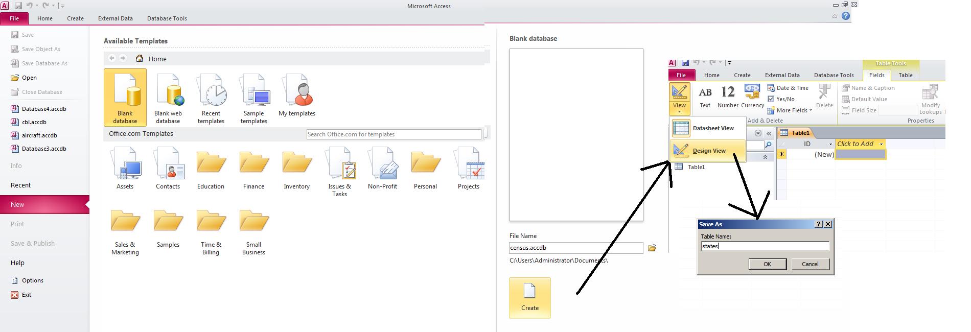
While you are not required to do this, we will move into design mode. Notice that ID is already set. It is an autonumber which means that each new row forces an id entry of the next number. Autonumber is a large integer which means that it can go up to 2 billion in value and this should tell you the number of rows that an access table can handle. In other databases, a different technique is used based on the time and date of entry and this substantially increases the number of entries per table that are allowed. Click at autonumber and you will see a variety of types. Remember, once a type is selected, the data fro the column must conform to that type.

Now, let's set up the column state which is the state name. Besides selecting type, below you will see a grid which allows subentries. For text, a subentry is length of field. Access defaults to 255, No state name is that long so let's move this back to 30. In addition, there is a requirement for an entry and we should set that.
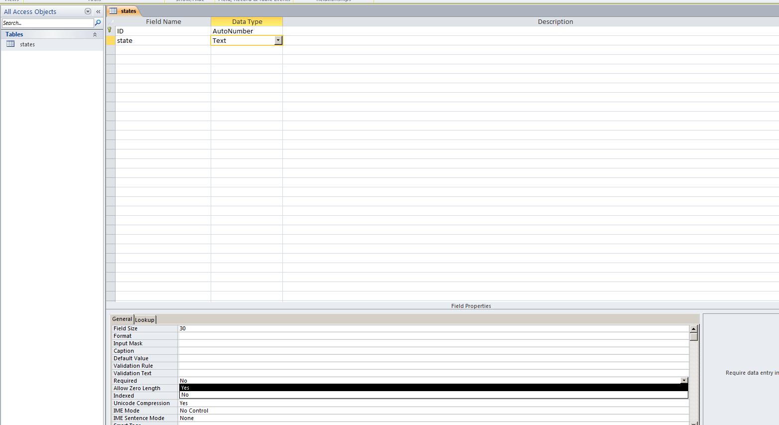
We now have three numeric fields to create, pop2010, change and pop2000. On all of these we should set the type of nummeric to long integer. It should be clear that all these entries do not need decimals but integer inself supports numbers to 64K. Long integer supports numbers up to 2 billion as indicated above. Below, we show this.
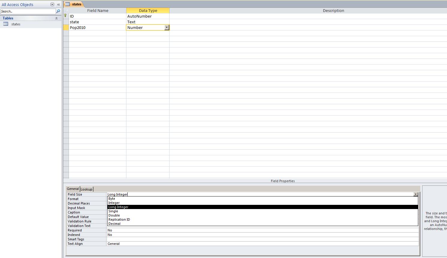
When done with design, we need to put in the data. Below we start this process by requesting datasheet view.
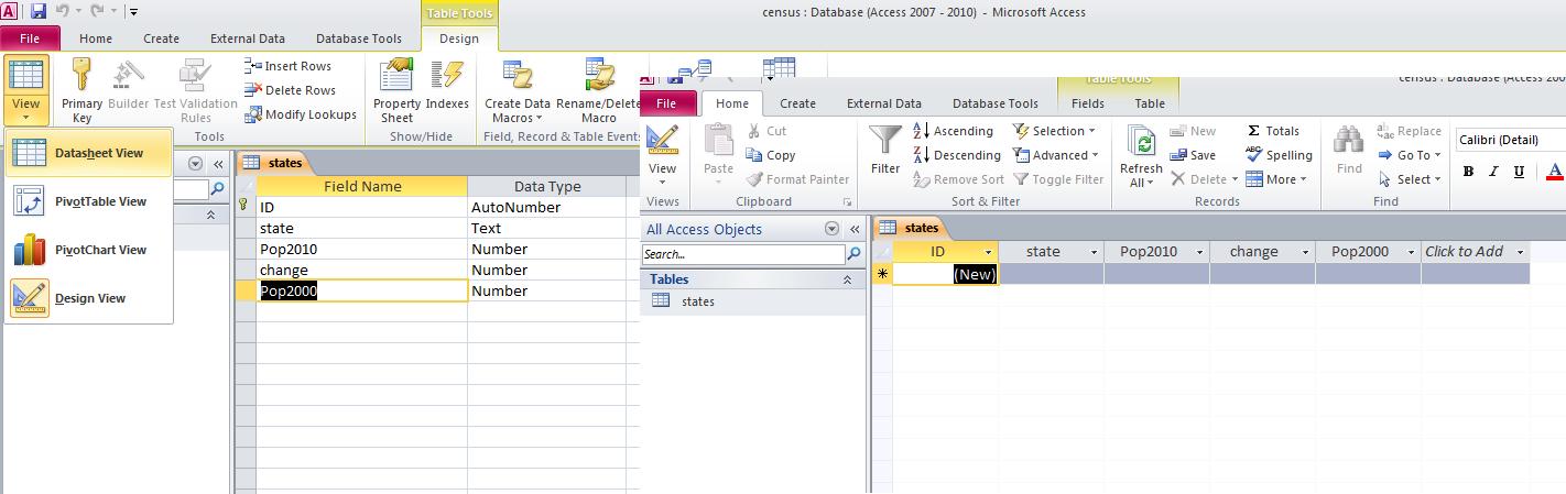
As I am recovering from what what turned out to be a worse operation than expected, you should have a guest instrcutor today. Probably, it will be Charles Herbert, the Computer Technology dapartment head, although may be someone else. Whomever it is, please afford them the hospitality of our class and listen to them as this is our last lecture in Word.
Let's first handle where we go from here. We need to discuss your test and my hope is that by Tuesday I have an idea of what this will entail. I am aiming at a Friday debut of this and will give you more details as we go along the week. Whatever, the test will be online using the myitlab site.
Given that we are about a week beyond where I expected to be, I think we will deal with Access first and then Excel although I will make a final decision on Tuesday. If we go this route, your test for Access will be combined with a question or two from our discussion of the internet and communications (the first 2 weeks) in a take home that I will create as we finish Access - I expect a two week discussion of such. In additon, since we will be dealing with databases, I will try to get Library services to give its lecture during this time. Enough of where we are going - and as said final determination will be decided as of Tuesday - and onto today's lecture, the last of Word.
Let's access our file by clicking here. For the Monday-Friday class (11:15 to 1:05), we ended the lecture last week with an attempt at a pulled quote. First there was an attempt at bulleting and numbering. So, the next few commands and actions should be attempted by the Mon-Wed class (2:30 to 4:20).
About page 7, there should be a list of TV parts played by Patrick McGoohan. If not on 7, you can find this by searching for the text TV parts played by . See the list? Let's bullet these. In the paragraph group, the top left command is a bullet. Select the 4 paragraphs of TV roles and click on bullet. This is the generic bullet. Yopu could also number. Click on the command next to the bullet command. Now you see generic numbers. Bullets and numbers can be enhanced. Notice the added conrtrol to the right of the command. Clicking this gives more options. Let's keep it as number.
We had highlighted a segment of the word document we were using bounded by TV parts played by Patrick McGoohan to Capt Rafferty in Rafferty. We could find this by scanning the document or by using the find instructions that we have studied. Now, I do have a problem. This was not done in the Mon-Wed class given the network outage we had at the beginning of Wednesday's class. So, in loading our document, I have provided both the straight text and text within a textbox and your instructor can decide where to begin the lecture. Below, we show in a set of composite shots what is needed per at least the Mon-Wed class: pulling this text into a textbox.
Now, for both classes, academic word processing needs quite a bit of footnote and endnote support. We will let our instructor handle how to do these things and at the beginning of your next class, I will bring in some books to show why we need these things. But, let's handle what we can handle today so I am copying below the portion of the lecture I did not get to from our last class.
One aspect of academic articles pertains to footnotes and endnotes. Assume you have some extra info you would like to indicate. Readability becomes an issue. You can handle this the use of footnote and endnote which allows the reader the option of looking at this extra info. Use find to fond the first instance of Ian Fleming although you probably can see this on the first page. Move your cursor after the g of fleming and go into reference and click footnote. Notice that a 1 is placed where you were and an area between the document and the bottom margin is opened. Notice the superscript 1 down there also. Type in the following. Ian Fleming, the creator of James Bond, was the grandson of Robert Fleming, who in the mid 1800's was the richest man in the British EMpire. He made his fortune investing in American Railroads.
Use find to find the first instance scarecrow. This should be on page 2. After the words, the scarecrow of Rodney Marsh, let's insert another footnote that indicates that McGoohan played Dr Syn, a simple country priest who led an insurrection against the British monarch. Notice that this is footnote 2. The system keeps track of this numbering.
Footnotes can be made into endnotes very quickly. Click your right button and choose note options. On the dialog box, click convert and then into endnotes. Below, we composite this process
An important addition ot the 2007 version of Word is the manage sources or bibliography section of the reference tab. It has even been upgraded from 2007. When doing a paper for an instructor, your instructor will inform you of how (s)he wants the citations - these are the sources you are using - to be listed. In the citations and bibliography group of the reference tab, click styles. You should see things like APA fifth edition, GOST, Chicago, etc. To use this, we need to put in several citations and we need to discuss (although the librarian will extend this discussion) what you are not supposed to do. And what you are not supposed to do is just copy info without indicating a source. This is called plagiarism and is seriously frowned on in Academia and can lead to you getting an F in a course. So, given the sources that you have used, howe do you load them into MS Word. While no true sources was really used in this documentation by your instructor who is the real author of this - and this is a sad situation for someone who is supposed to be a technical expert given that what you are reading about media is probably the only thing he really is an expert in - but here's some possible sourses:
Now, armed with these 2 citations, lets put these in a citations. There are several, but to your instructor, the easiest way is to click manage sources. The system will attempt to hold these sources for you for future projects and when you save the document. You wuill notice a left and right side. The left side is for previous citations you may have done. The right side is for the citations that you have entered for the document in question. Previous citations can be moved over by arrow to make them available for this document, but in our case we will need to enter the citation so click new.
At the top, there is type of siurce which defaults to book. The entries may change depending on the type of source you choose. If you click the check box to show all the bibliography fields, you will see they are quite extensive but it is easier to click it on again and use the fields indicated per your choice. Now, for book, using the two citations indicated above, enter the author, title, year, city of the publisher and the publisher year one at a time. After each one, click okay. Below we show our data prior to the addition of the second citation. You can see the first addition is set both at the right and left.
Generally, although not a hundred percent of the time, sources go at the end of a document. We already have table of figures at the end. Click ctrl end and lets add these sources to our document at the end. Choose the style that your instructor requests (for this class, let's use Chicago Fifteenth editon) and click bibliography. Choose either Bibliography or Works cited (this is similar to table of contents whre we chose either contents or table of contents) and with a clik these citations will be inserted into your document (Although the option insert bibliography will not put any title on for you).
Several things remain to finish this document. A quick discussion can be done on themes which you will find on the page layout tab. Themes organize the different colors being used in your document. Although we haven't used a great deal of color, look at page 0 (the cover page) (especially the line at the bottom) and the header on page 1 while selecting different themes under preview to see how colors are affected. This is new as of the 2007 version and corresponds to something that Powerpoint has had for the last several versions, We will see that in powerpoint, Microsoft has included something similar to this.
While on the page layout tab, you can also include a watermark. Either selecting an existing template or selecting custom watermark, you can add text or a picture. Let's use a text watermark and indicate For Educational purposes Only. Seelct a color (or leave it gray) and keep diagonal. Click Apply and you will see something similar to what's shown below. This is an example of what Microsoft calls Z-order which controls layering on the paper. Transparency in varying degrees is allowed and the effect here is a transparent watermark (or image) that bleeds through the text.
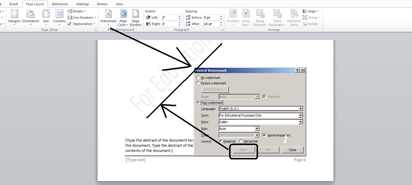
We end Word by dealing with several items in the review tab. We have already discusses research and the theseaurus in both classes, I believe. An important componebt is the spell checker which over the years has had a grammar checker added to it. Much is made of this facility, but you should understand it has a way to go. There is a famous poem that indicates this that you can access clicking here. Above the horizontal line is a correct syntax, below is a very incorrect syntax. Notice the spell checker runs through this as if correct syntax. Now, why? While misspelled in their use, all the words do exist and this throws off the grammar checker. Keep this in mind as you run this checker through our document.
At minimum the spell checker should find assumed misspellings per the proper names in the document. Patrick, McGoohan, Ian, Fleming, Goldfinger are not English words. These are proper nouns. To handle this, the program uses two dictionaries: one from the system designed for english, the other set by you as a custom dictionary. You can add to the custom dictionary on the fly as the spell/grammar checker does its thing or you can preset the proper nouns. Let's preset these 5 before running the checker. Click File, then options and then proofing as shown below in the composite.
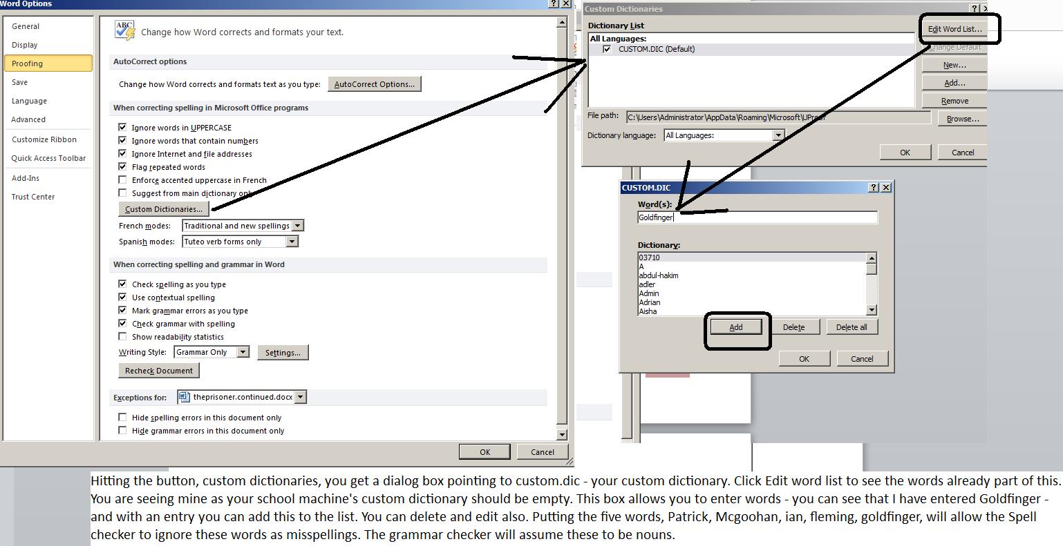
Once we've set these, let's run the spell checker although if set right the system is already dealing with this. As you look at the document as it has loaded, jagged red underlines are deemed to be spelling errors and jagged green underlines are deemed to be grammar errors. You can make changes even before invoking the checker, but the checker will give you options. Let's invoke it.
First, whereever you are the checker will revolve once around the document. If starting at the top this means straight top to bottom. If in the middle, it is down to the bottom, up to the top and then to the middle. Some text is shown and the error is indicated, this time in a straight red or green underline. Ignore once will allow you to proceed so that the error is ignored at this moment. Ignore all extends this so that during this launch of Word this error is ignored at all times. Add to dictionary involves adding this word to the custom dictionary (assuming a red line indicating spelling). Below the text is some possible algorithmically created substitutions and you can select whichever of these possible changes you want and through either the change or the change all (propagating this through the document), you can change this in the text. We will not discuss autocorrect in this class but it is an interesting secondary way to do spellchecking and you should study this otside of class. Below, you will see the spell checker has found Bourban, which is a misspelling for Bourbon. That spelling is below and selected and by clicking change all, we could wipe this misspelling off the document whereever it would reside.
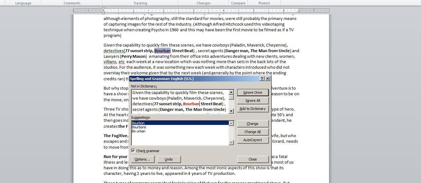
Finally, the comment, tracking and changes group combine several aspects of word processing the Microsoft has been working on with previous features of Word. This has been created to compete with Lotus Notes which allows group word processing. Assume three offices, Phila, Phoenix and LA and an attempt is being made to come up with a common letter used for a specific reason in all three offices. You might create the original draft, send it along to Phoenix who would make changes and they would send it to LA for changes before sending it back to you. You would want to see what changes were made and by who, rollback any changes you don't like and read any comments. This section allows you to do this. Your book doesn't indicate that this works best when a group is dealing with this and would be cumbersome for just one person. Remeber, you alone can use undo and redo to do much of this when crating your own unique document.
Start with show makeup. When in this section, you can control what type of changes or revisons to show and whether to show these changes, revisions and something called comments can be shown within the document or by balloon. Balloons are the standard choice and their use creates an additional panel to the right of your document where you can see these.
Let's start with comments. Assume that there is a question about whether the footnote for Ian Fleming should be included. Move your cursor to the suerscript 1 after Ian Fleming where you had set the footnote. In the review tab, click new comment. Notice the inclusion of the panel and the comment. Generally some indication of who is the author of the comment is indicated within the brackets. After the colon type in: Do we really need this footnote. Even before leaving this, go up to final:show markup. Switch between final show markup and final. Notice how the comment appears and disappears. Printing will do this also as the system, when printing the comment as a balloon, will decrease the zoom to a number lower than 100% (the norm for printing) to accomodate the ballon. Below, we catch a picture of this as we have gotten into the file menu and then print. Notice the bottom right indicating 84% of view allowing a portion of the document (at the right) to hold thge comment. Now, remember, this is being set for print with the final markup option as final show markup.
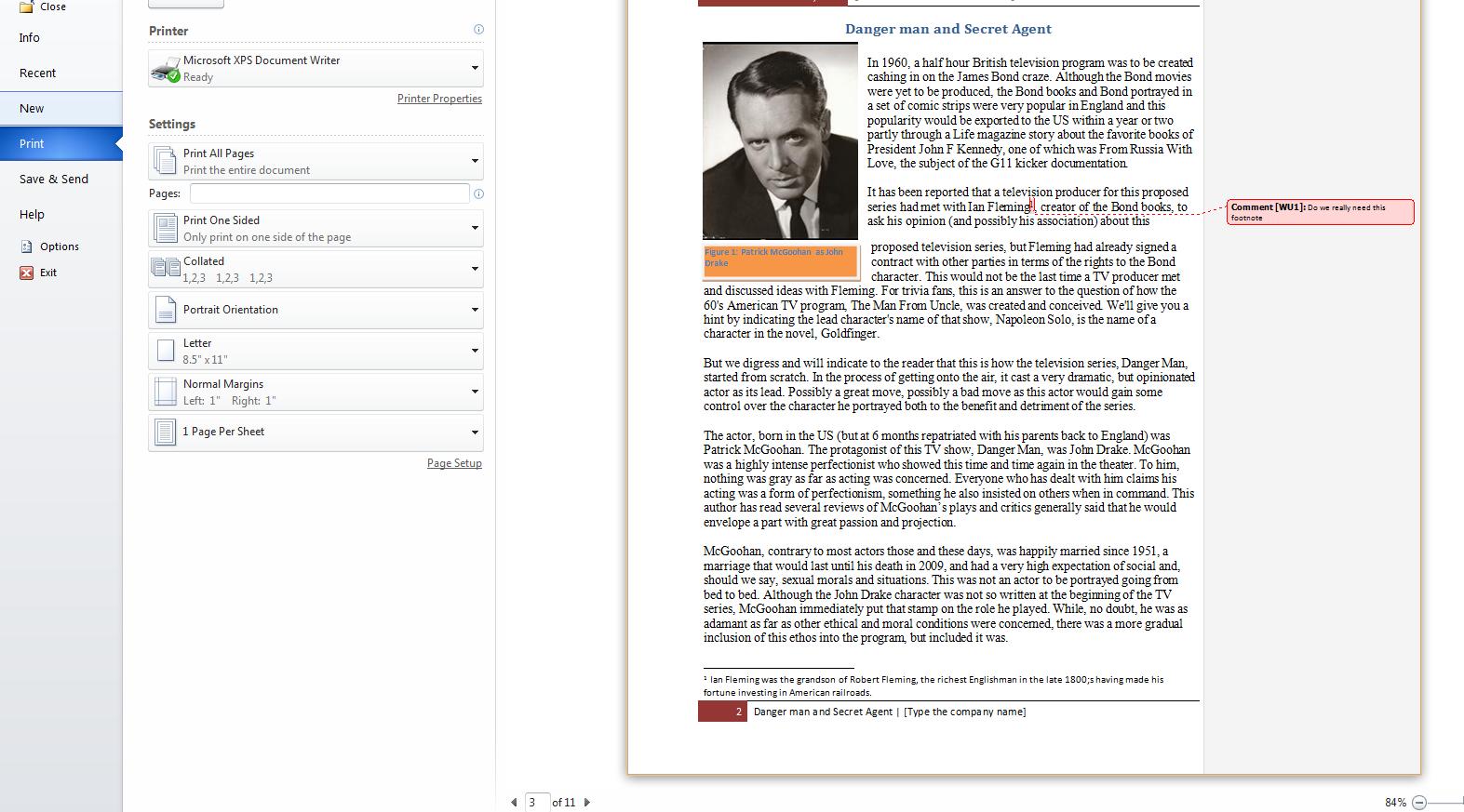
Now, go back to the review tab and click reviewing pane. This defaults to showing the reviewing pane vertically which results in another panel but this time to the left. This panel can do a lot of things including modifiying the text and changes in the body of the document. At the moment, only this comment is showing. But if you right click the indication of the comment in the reviewing pane, you could delete the comment, a type of rollback. Below, we show this.
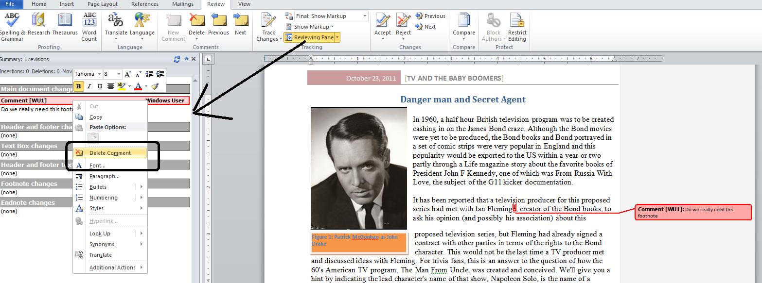
Now, this gets extended by track changes. This was originally used for legal documents but Microsoft has expanded this in concept. There are defaults that you can change but for our purposes just click it on by clicking on track changes as shown below. Now, right in this area is the line ask his opinion (and possibly his association) about this. Change this to his opinion and association about this which means you have added and association and deleted (a possibly his association). Notice our add is in red and underlined. Our deletion is in a balloon, Before doping anything else, go up again and click inside final:show markup. Final gives you the document as if track changes was not invoked. returning to final show markup, we see the comment and delete balloons and we see the red underlined addition. Notice also that the reviewing panel has been modified. Moving either to inserted or deleted on the reviewing panel, we can accept or reject the insertions which would alter the document (accept would set and association as the text that should be displayed and the delete balloon would disappear, reject would set the document back to what it was before our insertion and deletion)
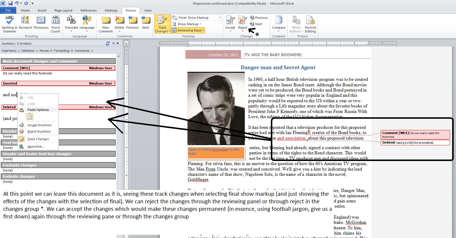
Since the reviewing pane also indicates the user who made the changes, you can see how you would be able to determine which office (if not user) made the change.
Today, we are going to deal with larger documents. This would not be a surprise given the Microsoft Press (the book publishing arm of Microsoft) forces authors to use Word on manuscript submissions. The document we will deal with at present has 8 pages. You can access it by clicking here.
First thing, today - navigation. You can try Ctrl home and ctrl end and you will find both work. You can also put in all the bookmarks you like and this will also work. What changes here is the need to cycle through pages, lines, objects, etc.
We'll start today with Goto which as discussed last lecture is part of the find/replace/goto dialog box. Let's get there. Select page and enter 4 and click goto. Below is a composite of this. Included is the abiltiy to increment or decrement and we'll do that in class, also.
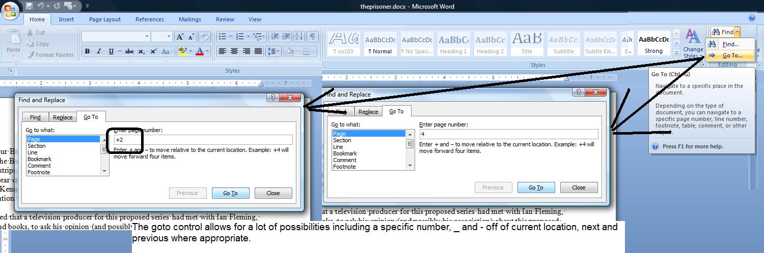
We'll look at the line count also. Let's head to line 200 and then decrement by 100. This takes us to page 6 and 3 respectively.
Now,let's add some pictures. Click the links and save the pictures to your computer. click for drake.jpg and Click for prisoner.jpg. Put both of these into the pictures folder.
Add the drake picture onto page 1 and the prosoner picture on page 4. Use either position or tight text wrap as we have done previously in class. You can move between pictures using goto if you would like. Make sure to click back into the document. Activate goto and play with next and previous and you will find that you can move between the two quite easily. Let's use this to set captions. You will remember that we set a caption on the last class under Michelle Pfieffer's picture. On the first picture, set a caption designated as Patrick McGoohan as John Drake. On the second set a caption as Patrick McGoohan as the Prisoner.
Word has a set of lists that you can create using the reference tab. One is a table of figures which is nothing more than a listing of the captions. Go to the end of the document and click reference and then click insert table of figures. The system is set to use links for this so set uncheck the check box so that we can see page numbers. Pick a format of your choosing and click OK, Below represents what we should be seeing.

Another possible list is Table Of Contents and in this versin of Word, it is merged with the navigation panel. At the beginning of the document, enter a new line - Origins of Danger man/Secret Agent. With your cursor still on this line, set the paragrasph style to heading1. Near the top of page 3, the document discusses the prisoner TV show. Enter a line - The Origins of The Prisoner. On page 5 you will see reference to - in the A13 and B13 documentation. Above this set the line - Adding the Saint. Again set this to heading1.
Now, two things. In the view tab, activate the navigation pane. You should see these added lines in the tab. For this version, the styles of heading1, heading2, headingx are shown in the navigation panel. Notice, that by clicking on these entries, you move to them. Now, let's add the list I was talking about. Create a new first page. The easiest way to do this is by Ctrl Home, Ctrl Enter, Ctrl Home. You should have a new page. Now, onto the reference tab. Click table of Contents and that's what you will get. By the way, word processing professionals designate this as TOC. Below, you see a table of contents with a navigation pane. One additional note: Use ctrl when clicking the TOC entry to move to it.
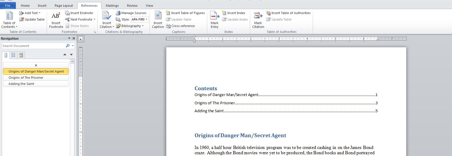
One aspect of academic articles pertains to footnotes and endnotes. Assume you have some extra info you would like to indicate. Readability becomes an issue. You can handle this the use of footnote and endnote which allows the reader the option of looking at this extra info. Use find to fond the first instance of Ian Fleming although you probably can see this on the first page. Move your cursor after the g of fleming and go into reference and click footnote. Notice that a 1 is placed where you were and an area between the document and the bottom margin is opened. Notice the superscript 1 down there also. Type in the following. Ian Fleming, the creator of James Bond, was the grandson of Robert Fleming, who in the mid 1800's was the richest man in the British EMpire. He made his fortune investing in American Railroads.
Use find to find the first instance scarecrow. This should be on page 2. After the words, the scarecrow of Rodney Marsh, let's insert another footnote that indicates that McGoohan played Dr Syn, a simple country priest who led an insurrection against the British monarch. Notice that this is footnote 2. The system keeps track of this numbering.
Footnotes can be made into endnotes very quickly. Click your right button and choose note options. On the dialog box, click convert and then into endnotes. Below, we composite this process

We had already indicated to you that there were pre configured cover pages in this system. This is designed to use the info in properties to create a new first page. Invoke a cover page through the insert tab. Notice that it will pick up several pieces of info from properties. Now, look at your table of contents and table of figures. The page numbers are not reflecting the addition of the cover page. Click you right button over the TOF and TOC and choose update field and then update page numbers to correct this.
Having invoked a cover page which is a template, let's look at headers and footers. Invoke your header either through a double click or clicking header in the insert tab. Pick austere even. Up in the header/footer tools, select different odd/even page. Also different first page. Notice that the header on shows on page 2 and 4, etc. Move to page three and invoke austere odd and now page 3,5 ,etc are set. On page 1, invoke Alphabet. Notice how you have different header selections. Below we show a composite of this.
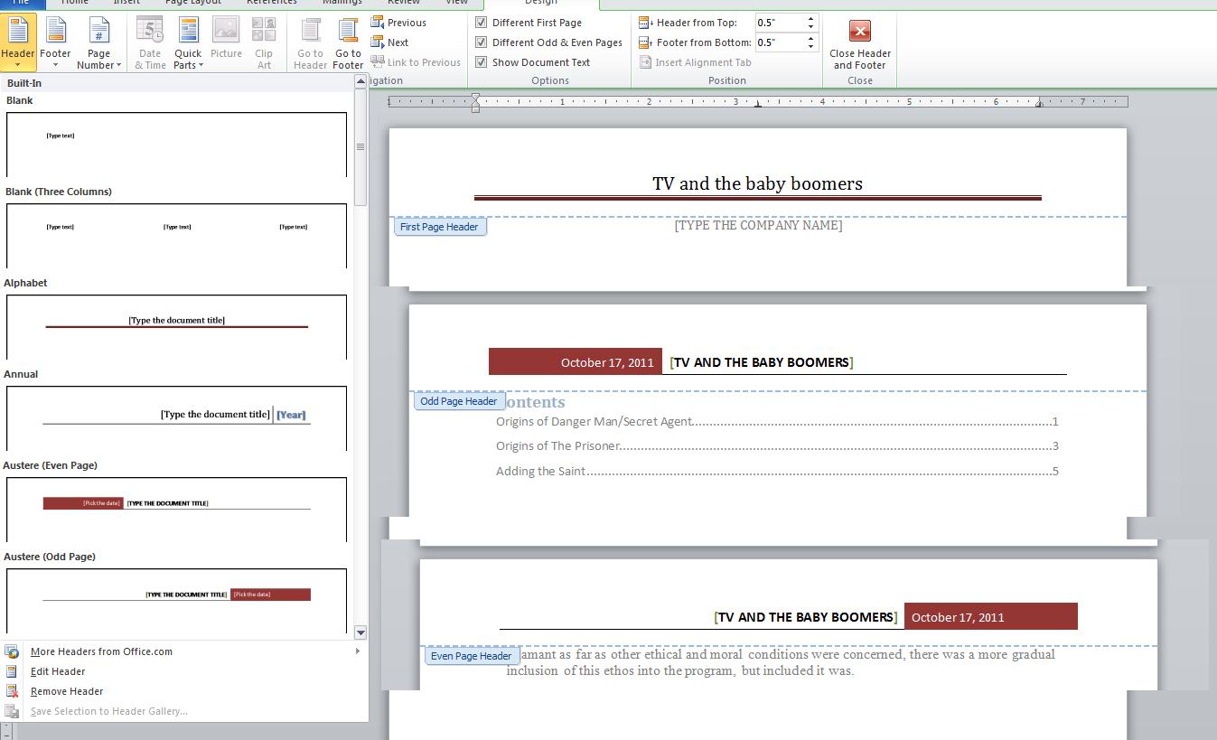
We can do a similar situation with footers. Pick austere odd for the odd pages and austere even for the even pages. And pick alphabet for page 1.
Before the origins of the prisoner is a list of TV roles of patrick McGoohan. Let's bullet these. In the paragraph group, the top left command is a bullet. Select the 4 paragraphs of TV roles and click on bullet. This is the generic bullet. Yopu could also number. Click on the command next to the bullet command. Now you see generic numbers. Bullets and numbers can be enhanced. Notice the added conrtrol to the right of the command. Clicking this gives more options. Let's keep it as number.
We are about to do a pull quote. Highlighted text when a text box is invoked will be placed in the textbox. Click the insert tab and then textbox and draw textbox. Notice that the text is now contained within the textbox. Textboxes can be reshaped. Click change shape in the textbox tab and select an hexagon. Add to this by some 3d options and color options. Below, we see an example.
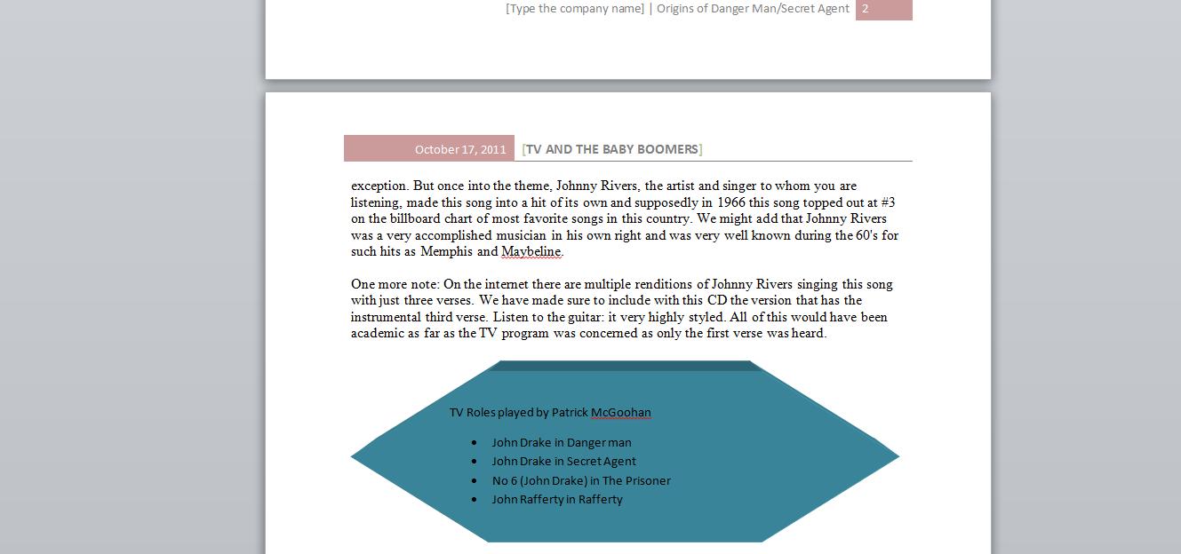
Several thing left to discuss. Citations under reference, spell checker and something special in this, spell, watermark themes, and changes to track changes (which includes comments) If we can do it today, we will but I think this is moved into the next class.
Our first order of business will be a discussion of a modified schedule due to my need to undergo some unexpected (and somewhat emergency) surgery this coming Thursday, Oct 20th. I'm not happy about this for multiple reasons including thae fact that I don't like to miss classes that I am teaching. If there was any way of getting around this, getting around this we would do but that's impossible. I'll be glad to give you all the gory details of this that you want but if there is any moral to this it would be: don't get old. In a nut shell, here's our modified schedule for the next week and a half.
Mon-Fri class: Meet today, Oct 14th amd Monday, Oct 17th. Off Fri, the 21st. Hopefully back on the 24th if the surgeon is accurate as to recovery.
Mon Wed Class:Meet Mon, Oct 17th and Wed, Oct 19th. Hopefully back on the 24th if the surgeon is accurate as to recovery
We are in essence done with the catacomb file. One or two things remain to do and then we want to look at things done per the entire document. In our next class, we shall use a much larger document, one with over 10 pages. But we can use this finalized catacomb document, which you can access by clicking here.
I have added the text boxes in the header. Selina Kyle's and Cat Emporium are contained within textboxes as straight text could not really be positioned there. The cube effect of that you see with Cat Emporium is done through 3D effect.
Normally, with a document such as this, I would try to get it onto 2 pages and not 3 as shown, but we are not that interested in this for this document.
But, what we are interested in is finishing this using some tools not yet discussed. One tool (but we will look at 2) that was discussed but not shown was indent (outdent) found within the paragraph group.
Indent works on all the lines of a paragraph and moves them through a tab set. If a tabset is not set, the default tabset of half an inch is assumed. Look at the paragraph below the classic day. select a part of it and a part of the paragraph below the grand escape. The picture below shows indent and outdent in operation.
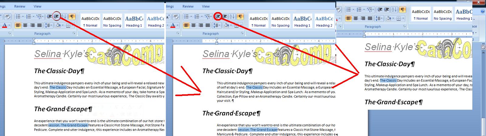
While your instructor is not a big fan of what is to be shown, and considers this remnants that exist from the typewriter age, you can set specific tab sets on your word document. This is a paragraph command so each paragraph where you would like to use thismust be prepped. Without these additonal tabs as will be shown, each paragraph defaults to a set of left tabs each half inch.
At the bottom of the paragraph dialog box is a button designated as tab. Click that and you will be on the tab dialog box. Notice that the default is half an inch. You can enter tabs and designate them left, right or center. Now, I'm going to do this on a separate line and emulate a row on a table where we have left justification, centering and right justification all at the same time. I should not that this is much easier using tables.
I will enter a 1.2 inch tab keeping the default of left. Next is a 4 inch center tab and finally a 5.5" right tab. the picture below shows this and the result.
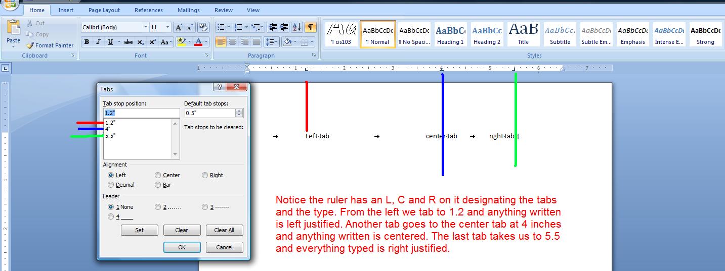
Let's see if we can center the classic day at 2.5 inches. Once the tab set is determined, move your cursor at the beginning of the line and then tab. Now, let's set a style for this. This is really normal with this additional tab set. Click for creation of a quick style and name this cis103 or whatever. You can just save this as there is no addtional layout commands to designate. Now, move to the grand escape. This is the normal style. Click the cis103 style. Notice that the centering tab is being displayed. Tab to it. You can repeat this through all the titles. You could also have used the format painter in this.
Now, let's assume that this marketing piece is going to be both mailed and Emailed. Email gives several new possibilities including the ability to link. We saw linking when we studied html and we are about to see this in a word document.
These treatments have been copied from Toppers Spa which is a spa treatment facility close to where I live. I've never used it but a friend's wife raves about it so I have no problems in telling you about it. Let's link the text, the classic day, to the website designated as www.toppersspa.com. Below we put in the hyperlink (which is just a computer term meaning link onto the internet) at the text, the classic spa. When done, you can invoke the link by control clicking on the link whicgh is different from web usage. Notice, however, similar to the web is the underline indicating a link. And, finally, note that this makes no sense if this is printed and hyperlinks are not indicated when on paper.
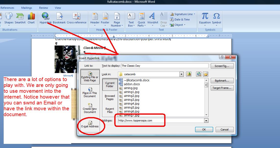
Let's assume that we would like to link within a document. Or, perhaps we know that we will be back to that area to do more work. There is a set of internal links in Word designated as bookmarks. Normally this is used with larger document and we probably will revisit this next we meet when dealing with a really multipage document, but while we are talking about links, let's set a bookmark.
Place your cursor where the bookmark should be. In this case at the text, the classic day. Onto the insert tab and bookmark. Bookmarks do not allow for embedded blanks so you may use an underscore or just ignore spacing. I am going to type aclassicday here and click add. If we come back to bookmarks again we will see aclassicday and clicking goto will take you directly there. But we want to link within the document. Highlight the paragraph we bordered and click insert/hyperlink. Now, instead of a web address, click with the document and the book,arks will show up. Indicate aclassicday and then click OK. If done right, we should see the text underlined and clicking on the text will take us to that spot. Below we see the creation of the bookmark.
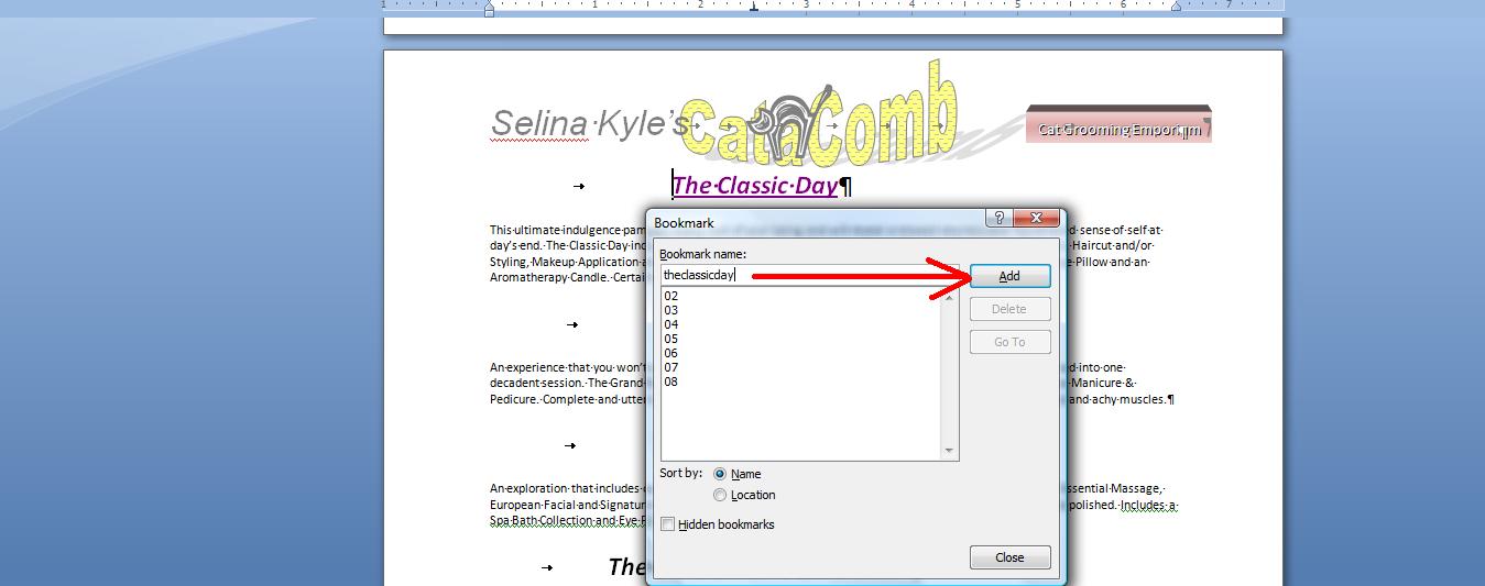
Now, while we have a small document, let's concentrate on several things that we can readily see although these techniques will work on large document as you will see next class. The first thing is search and search and replace Word describes this as find and find and replace. For small documents, searching would seem trivial but it does have its purposes as you will see. In the home tab, look to the right under editing and you will see find/replace and select. Find, by itself, in this version takes you to something new for this version, navigation. This will list out all the occurrences of Selina as you can see below. Ypu can either navigate to these by vlicking or cycle through using the up and down arrow. Assumptions are made here as to ignoring case and location.
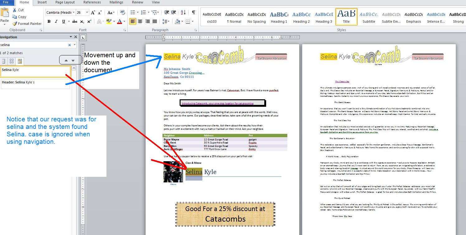 Notice, there is a designation of advanced find in the find control. In essence, advanced find and replace (and goto under find) take you to the same place, a dialog box with several tabs as indicated below.
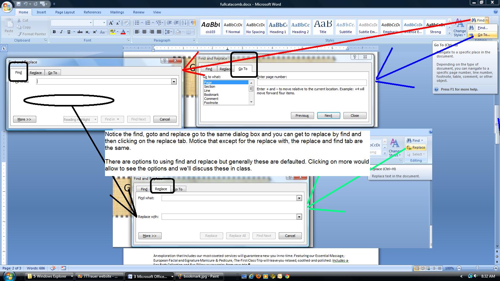
You can use this advanced find to search for selina and you will notice it cycles you around the document. There is a more button. Clicking this gives you more control. You can search by case (which in word processing means capital or non capped letters) and you can make sure that whatever is found is a word assuming you submit a word for the search process. In class I will explain the other options but these are very rarely dealt with. Below are two buttons which can be very useful. Format will allow you to add format options to your search and even allows you to just look for format if your search entry is missing. Special allows you to search for several special characters. So, if we were to click match case, we would need to enter Selina to find a match.
Now, let's assume that we are trying to replace Selina with Salina. We could use the navigation search or the find to find each instance and then change it by typing. A faster solution is to use replace and you should click on the replace tab. type in selina for find and type in Salina for replace. Notice the cap S. Click replace all and you should see 2 replacements and when done the changes should be a part of the document. And, by the way, since we specified a specific Salina, we should see that S capped on the replacements.
Since we are dealing with caps, we might as well indicate to you that Word supports 5 types of cap indication. Some of these should be obvious: small, larges, title (capping the first letter of every word). Not so obvious is sentence and toggle. You can see these in the font group, Aa control. We'll do a few for you in class.
Before we end with some proffing tools, look at our picture. Notice the meow below the picture. The meow is in a text box which you could put in your self. It is easier to do the first of several operations we will use the reference tab for. Click on the picture and click the reference tab. What you are seeing under the picture is a caption. Let's set another. Click insert caption and you will see the caption dialog box probably designated a figure 1. Put something in the text box and tyhen click okay. Notice that the caption is now what you just saw. Captions are a special form of text box and once set you can use text box tools to further enhance them.
Final thing for today. Take a look at the review tab and the proofing tools. We will be dealing with this either end of today or next time we meet using a different document. We have spelling and grammar, research and Thesaurus. Let's start with research. While working on word and being connected to the internet, you can access sources controlled by Microsoft including Bing which is a search service jointly operated by Yahoo and Microsoft. Now, the other things: Thesaurus, spell and grammar checker will be explained in either this class or our next class.
We would like to finish the Catacomb problem. What remains is to add some text (some of which has already been added to the file), add a table and add some text from a file and in that text deal with bullets (and numbers). When done, we should check or spelling and grammar. The file as we left it last week can be accessed by clicking here
Right before the picture, we should create a table. The table contains several names supposedly of clients. You will see enough tables as we deal with Excel in the future and you already know that you can, through OLE, invoke an excel spreadsheet through Word.
We however will deal with Word tables. This is not as extensive as Excel and while the program gives you some capability for math in Word tables, I've never been able to adequately control the math and, if it is me, I use Word tables only for styling as we will do here.
A table is made up of rows crisscrossed by columns. At the intersection of each row and column is a cell. A cell acts like a little document and you can do just about anything in that cell that you would do in a document (including adding another table) except tab as tab is the tables way of moving from one cell to another. What is of interest on a row, for instance, is how you can left justify one cell, center another and right justify a third. And, this may sould familiar as this is how your header and footer work which really are tables in disguise.
Before doing our table in this doucment, create a new document in word. Remember, you can switch back and forth between documents either through the status bar of the operating system or through view/switch windows control on the view tab.
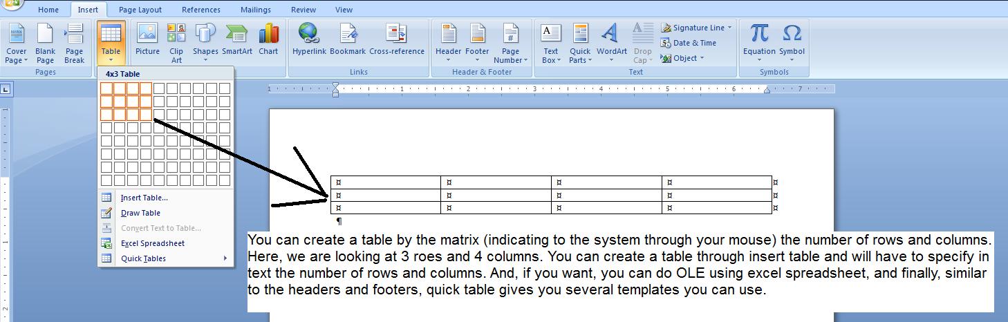
You can use your mouse to move to a cell or use the tab key to go to the next cell however be ware that use of the tab key in the last cell duplicates the last row (which is added).
Tables can be zoned and by that I mean that you have selection capability. With you mouse depressed, move your mouse cursor through the first 2 cells. Notice how both are selected. Now, with your ctrl key depressed, add the last 2 cells to your selection.
Rows can be selected by moving your cursor slightly to the right of the row and clicking. Keeping you mouse depressed you can add other rows (up or down) to the selection.
Similarly, you can select a column by moving your cursor slightly above the column and you will see a smll arrow. Click and that column is selected and similar ot rows, multiple columns can be selected.
Finally, every time you have been over the table, a little square has appeared top left of the table. This can be clicked to select all the cells of the table. Right clicking this control will give you many other options.
Let's run a little exercise. For each cell, type in the text of it's number. Cell one has text of one, cell two has text of two, One through four should be row 1, five through eight should be row 2 and nine through twelve should be row 3.
Now, do the following. Select column 1 and underline. Notice how only column 1 is underlined. Center column 2. Bold and set as 18 point size column 3. right justify and color column 4's text in red. (notice that all color is directed to the text) Below, we have done this.
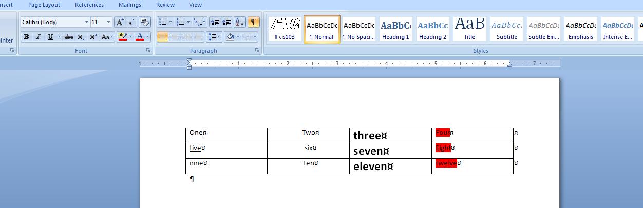
Background color for thec table is provided by extensive formatting and layout options which are available to you within the layout tab. Below, here are some possibilities.
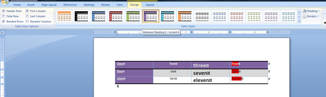
Now, having done this, we want to return to our catacomb document, the other document in Word. We need to insert the table as indicated below.
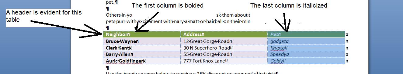
Let's do this. Create a 5 row by 3 column table. The first row is a header so click header on the header check box in design. Fill out the data. Click the first column and bold. Click the last column and italicize. Finally, use layout to select an appropriate design (or layout) for the entire table.
We are into the second page. The second page info is in a file. Before bring up the file, we need to create a second page. This is most easily done by using ctrl end to go to the bottom of the page and then clicking ctrl enter to create a page break. You can also clikc page break on the insert tab. Notice, as you create the new page that the header is automatically copied. This is what we mean by headers and footers. They are on all the pages (with some control) and you don't have to worry about placing them separately as pages are addded. And, if using page number, the numbers are automatically set for you.
We need to move this added document onto your socument section. click here to load this text. This is now the 3rd word document you launch of Word is dealing with. Npw, use save as to save the document to the document directory of your system.
Move back into the new page. Remember how we ran Excel through OLE. Microsoft has added another oprion under object: text from file which is added to the document. Let's invoke this and read in the file you just saved. Below shows my document after loading the addon text.
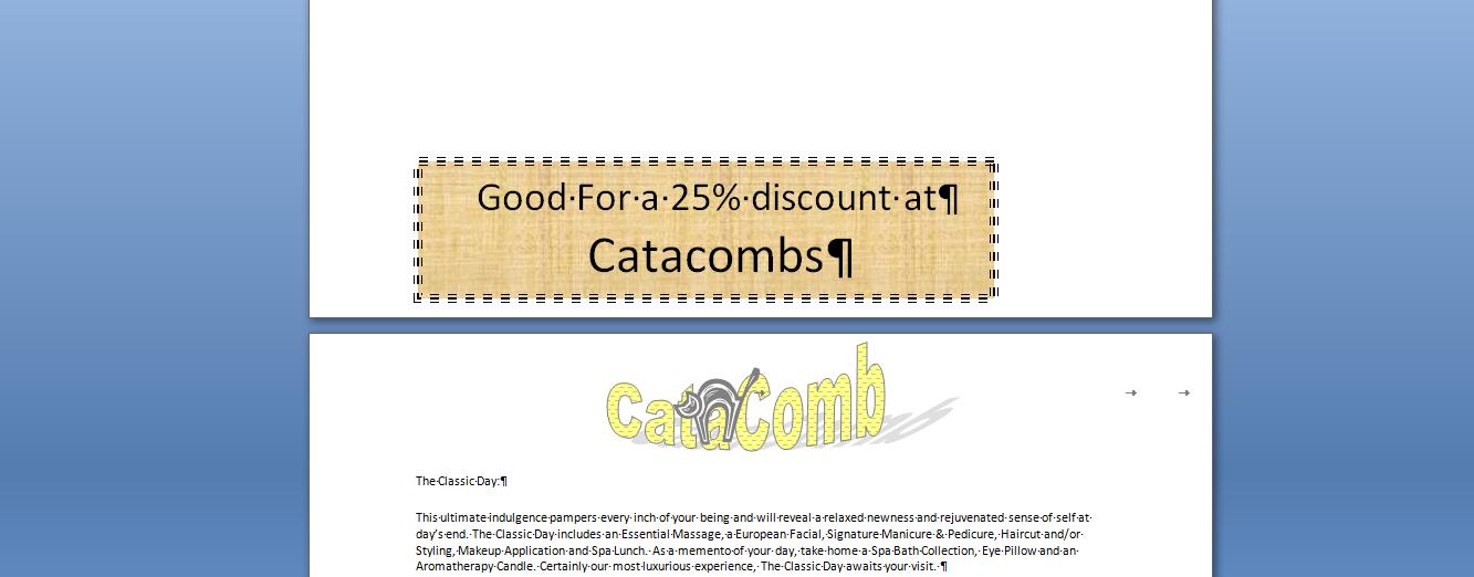
Now, this page looks relatively drab. We can do some things with it. Take the first offer, The classic day. Let's set this to Calibri 18, bolded and with 6 pts of space afterward, none before. We hope that wasn't hard given your participation in the class, but notice there are 6 more of these to do. Do we have to do each of these the same way. Isn't there some way to copy format just as there is a way to copy text. Yes, and there are really 2 ways. Let's work on the first way.
In the clipboard group is an icon designated a format painter. When clickng this, it is expected that your cursor at that point resides on something whose format you would like to copy. This is the paragraph, "A Classic Day", is it not. Move your cursor anywhere on this paragraph. When format painter is clicked, it tries to determine all the characteristics of the text and paragraph where the cursor was. Now, move your cursor over the document. Notice that the mouse icon has changed. It looks like a paintbrush. Highlight the text you want to reformat. When you let your mouse button go, these format changes will be applied to the text (and the paragraph). Let's try this for the grand escape. The grand escape text should look like the format of the classic day.
This works very well when there is a need for small changes. We have 6 or 7 of these paragraphs to change. What if we had 50? While better than setting each paragraph separately, it still would be a long process. For this we need styles.
You can see the already existing styles within the styles group. Originally, styles were paragraph oriented but in recent versions they have an indicator as to whether they should be paragraph, character or both. To see the charactieristics of a style, click your right mouse button over the style and select modify. Let's use the normal (or first) style. right clicking you can see that this is paragraph oriented and the preview tells you the characteristics of the style. Let's do the following. Using normal, let's create a new style we will call cis103. Below, we start this creation.
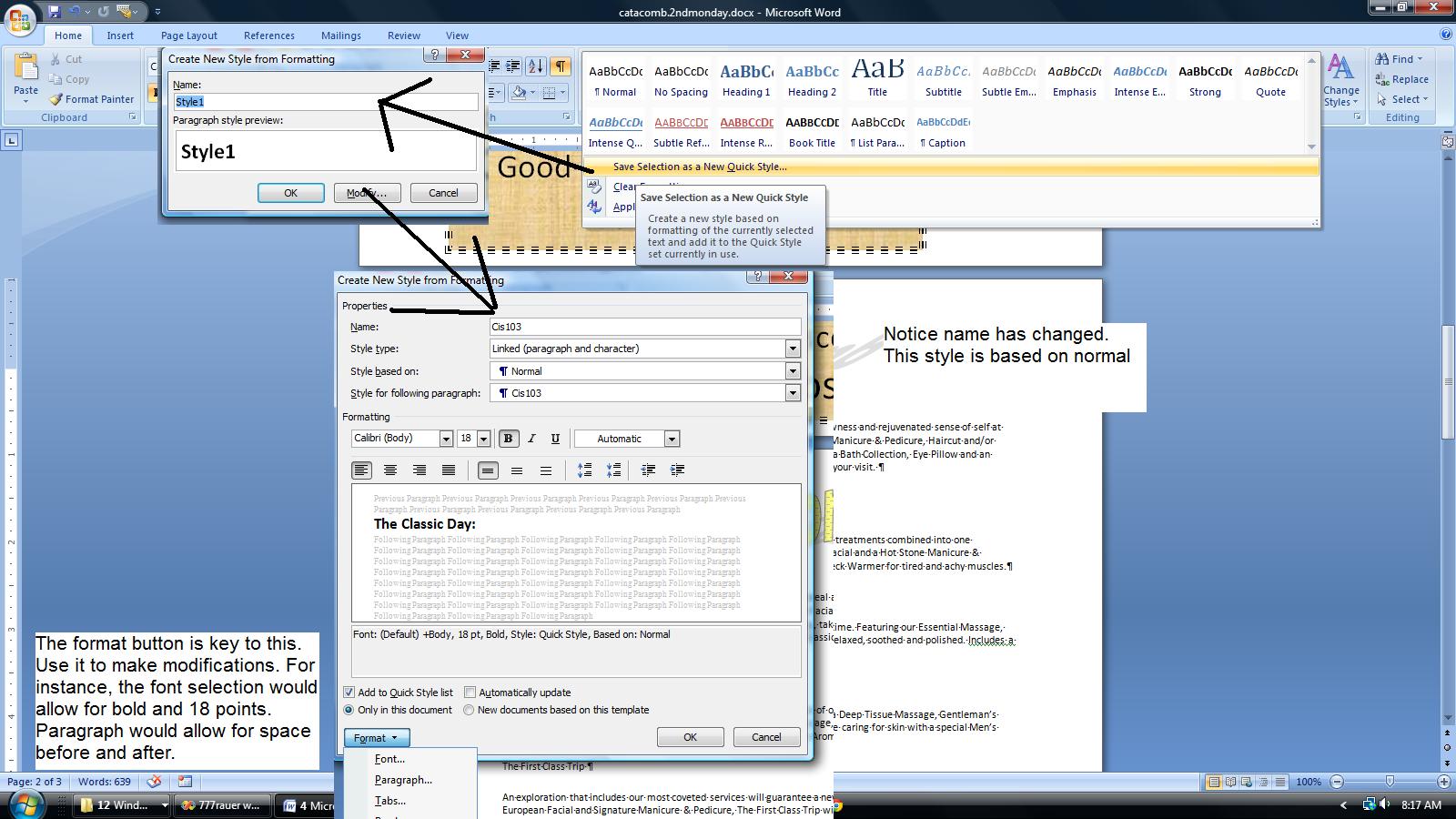
In addition, click the shortcut key. We ban use this to assign a special key set to activate this style. Use alt (alt is free throughout) and the letter c as we will name this style, cis103. Come back and save this selection. Move to the paragraphs in question. If done correctly, you should be able to move your cursor on a paragraph and click the cis103 style or to move to a paragraph and use ctrl C. Keep in mind, somethines the system gets confused. There is a clear formatting option on the style dropdown and you may need to apply this first before applying this new style.
If we have time I would like to run the spell and grammar checker. How accurate are these. do you think. Let's test it out with file you can access by clicking here.
As you should be continuing to work on the book's Aspen Fall Library project, we continue with the catacomb project. On Monday we added to our document and you can load this by clicking here.
As we load this up, look and you will see a date. First, this was saved as if Monday, but now it is displaying (at least we hope) today's date. But in addition. for the Mon-Fri class, we need to discuss the insertion of dates.
We want to enter a date as the first line. Hit the enter key to move the address block down further. Now, click the insert tab and click date and time. Dates (and times) can be entered in 2 ways. One is hard wired so that the specific date picked always shows up. The other is by macro, so that the date is picked up from the system and inserted. The update automatically chaeck box handles this for you. The available formats come from the operating system and dates have designation of short, medium and long and you can see this as we have 10/7/11, 10/7/2011,Oct 7, 2011 and Friday, October 7, 2011. Pick the date format you want to show and double click it to insert it. I'll let you decide whether this is a macro date or specific date.
We want to move both up and down through the document. Let's start with header/footers. From a previous discussion, you are aware that there are already pre-packaged header/footers in this system. We are going to create our own using two objects, word art and clip art.
We would like to handle the header. The 2007 (and this) version has really changed how Word looks at headers and footers. In a previous class we looked at a predefined header and how it took info from the document properties and used it. Everything is different including how to access the header. You can if you want click the insert tab and then header. It is easier to double click in the header location to invoke this.
When in the header the system helps you with a new tab, the header and footer tool. You can see in this tool a set of controls that are of use for the header (and footer). Included are these preset header and footer objects. Date is included as is page number although both of these (you are already aware of date) are in the insert tab options. Access to pictures and clip art are also are allowed although again you can use the insert tab of the ribbon for this. Notice that you can also close the header and this would bring you back to the document although it is easier to just double click within the body of the document.
In the Aspen Falls problem, there is a use of clip art in the body of the document. we are going to do the same but just place it into the header instead. We are going to complicate this procedure by intermingling the clip art object with a word art object.
Now, what is word art. It is a cariculture of letters. Below, we track the process of putting a Word art object indicating catacomb into the header with this note: Using this document which was created in Word 2007, the access of word art will look different than what you would see with a new 2010 document. If we have time, I will show you how to get to the same conclusion using the 2010 controls.
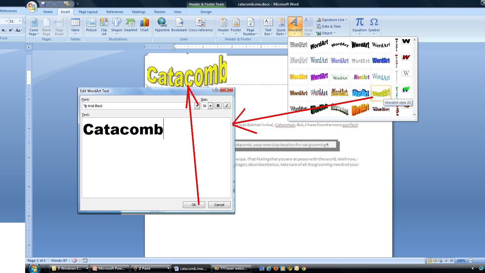
Not shown here is the invokation of an additional tab, designated as Word art tools. If on the word art object, word art tools will show up. if on the header, the header footer tools tab is in operation. Now, on the word art tools, let's look at this. You can space out or compress the letters. You can change the style. In addition you can change the color of the inside (known as a fill) and the outside (known as the border) of the characters. You can even change the intrinsic shape of the style although this style was chosen as it looks like a cat as it scratches (you have to be both a cat lover and have clawed furniture to fully appreciate this).
Take a look at text wrapping. When we study the insertion of pictures we will delve into this and position more fully but for now, click text wrapping and choose tight. This will move the object somewhat. Move your cursor over calacomb and look for a 4 pointed arrow and when you see it, move the object with your mouse as the left button is depressed. Below, we have put this into position.
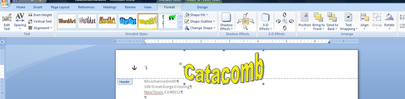
Wordart provides 2 additional controls with the picture on the document. A green circle and a yellow diamond. The green round circle will be seen with every object that is picture-like. For you navy types, this controls yaw, a term for swinging around an axis. We can try it in class. The diamond increases and decreases size on the horizontal axis. We can manipulate the diamond also but the optimal look is what you have.
Now, back to the header footer tab. Click clip art and a panal will open to your right. Let;s find a cat and so enter cats as the search for. Nothing is more beautiful that jet black cats (in their opinion also) so let's look for a Halloween cat and you can see that I have selected this in the screen shot below.
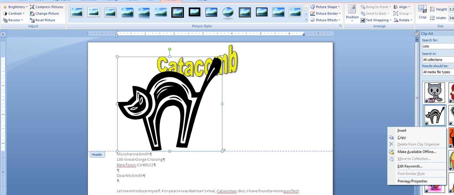
All right. Similar to the previous object, you have a new tab associated with this clip art (although it will probably say picture). Enter the tab and move to wrap text and set this to tight. Now, move your cursor above one of the four handles at each ofg the corners. You should see a 45% grabber. Move this in till the cat is an eighth of the original size. Move your cursor over the cat un til you see a 4 cornered arrow. Depress your left button of the mouse and move the cat so that it straddles the second C of catacomb as indicated below.
In placing the cat over the word art, we have obscured the fact that there are two objects here. You already know how to select an object - click on it. You can extend your selection (just as we extend selection of text) by depressing the control key while clicking. Use this approach to select both of these objects at the same time. If you have problems, your instructor can help you.
We are in an interesting position.We don't have the time to fully deal with this but a major extension of Word includes the building block/quick parts addition. We can save these objects as a header/footer and use them with one click in new document. How? Click quick parts and ask to save to quick part gallery. A composite sketch of this is below.
You can bring this back in a new document very easily. Below, we show you the entire header (we have truncated this for you in this problem) where a word art/clip art and 2 text boxes were used for the header and saved to quick parts and then recovered as a header on a new document.
Let's head south, now, and deal with spacing within a paragraph and before and after a paragraph. Hopefully, after this discussion, you will see that something is wrong on what is called the address block.
so, let's look at spacing. There is spacing within the paragraph (between each line). spacing before a paragraph and spacing after. Quite frankly, this is one of the hardest things to control in Word. It is complicated by another factor, the difference in size between the default fonts of 2003 and before and the default font of this and the 2007 version.
Let's take a look at the spacing options. They are part of the paragraph group which should tell you how they can be controlled. Below, is what we would see when this control is pressed. In addition, you can use the dialog box that the group is associated with.
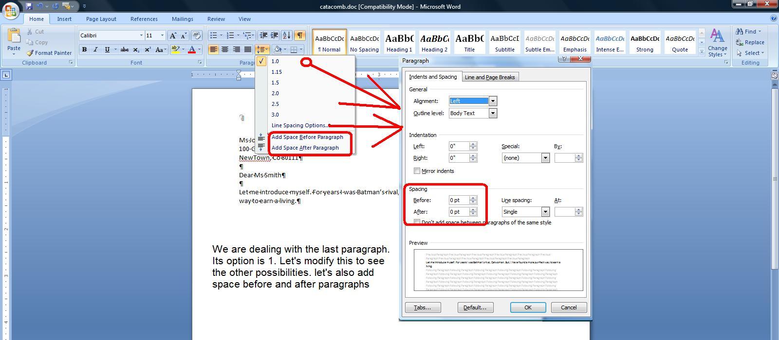
Most of the line options make sense except for 1.15. Can you guess what that might be used for. We'll give you a hint! In Office 1997 and 2000 the default font was Times Roman 12. In XP(2001) and 2003, the default fon t was Arial 10. In class we indicated that the heights of these two default font/point sizes were about the same. the 2007 and this version has a default of Calibri 11 which is about 7/8th smaller than the previous defalts. 1,15 is the fudge factor between the two.
If dealing with spacing within a paragraph, only paragraphs with multiple lines need apply. In discussing the question of spacing between paragraphs, you are dealing with spacing before and after the paragraph. It gets somewhat more confusing as Word gives you a further control which allows you to differenciate the apacing depending on the characteristics of the two paragraphs in question. We don;t have the time, and your book does not, to go through all this. But we do have to discuss this. Below is a sampling of within paragraph spacing including something called leading.
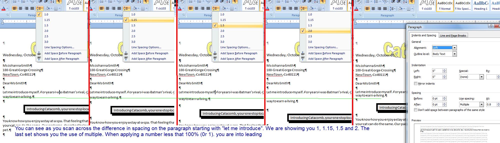
Now, what about the address block. If you want to set the address block to a line and a half (1.5) spacing, you would need to select the top 2 paragraph and apply 1.5. If you need to add space before or after the address block, it can be applied only once. You would need to select the first of the address block's paragraphs and set spacing before and the last of the address block's paragraphs and set spacing below. it would be easier if you could get the address block to act like a paragraph so that you can do this with one set of commands. You should understand that there are variations of your enter key. You have already used the enter key to indicate paragraphs. Sometime in the future we will be using a document that is more extensive and we will have need of page breaks. Whereever you are on this document, depress the enter while the ctrl key is depressed. You will see a page break created at this point. This is called a hard page break as you, the user, have created it. Page breaks instituted by the Word program are designated as soft page breaks. By the way, this answers why word wrap points are sometimes designated as soft returns and your enter key is sometimes called a hard return. use your undo to make the page break disappear.
One more use of enter is in conjunction with the shift key. This is a non paragraph break. In Internet terms, this is a <br /> as opposed to a </p> if this makes sense to you. Now, for the first two paragraph of the address block, substitute a shift-return for the return. Now, there are several ways to handle what we want to do. The spacing control in the paragraph group will now work on all the lines. Included in this contro; is spacing before and after. You would need 3 shots at this control to do everything. Or, you can go to the dialog box of the paragraph group and handle4 this all at once as indicated below.
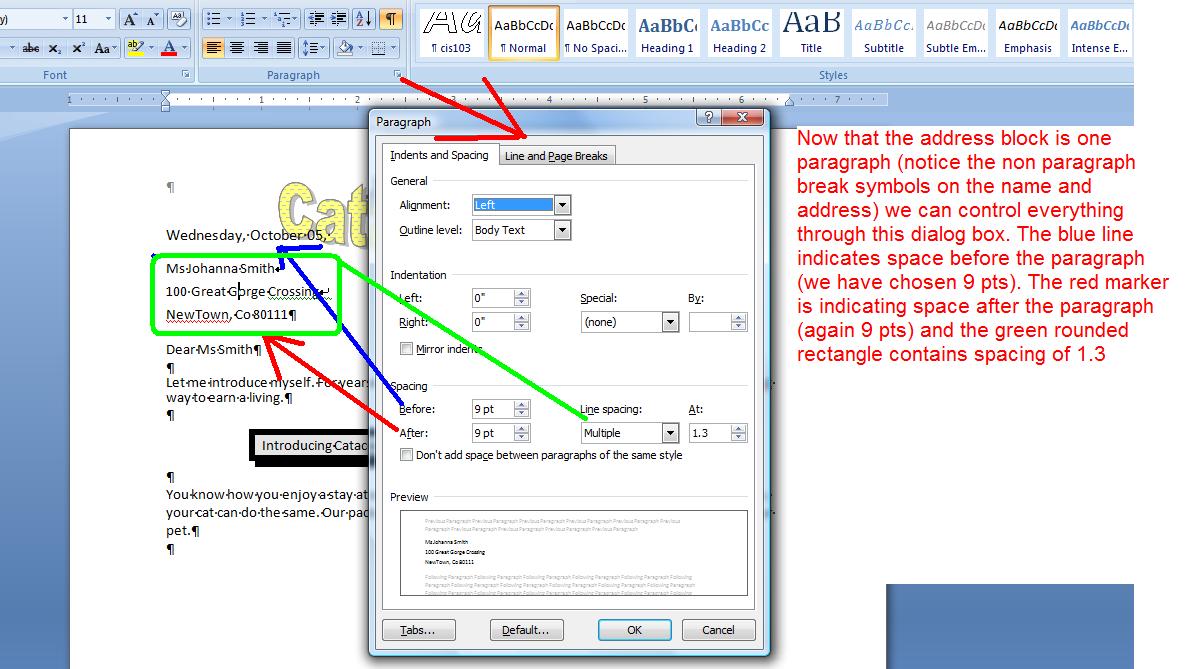
We will handle the table next class. For this class, let's enter the picture and this picture, by the way, is of Michelle Pfiefer when she played Catwoman in Batman 2 or 3. Notice the spacing and layout here. Caio and Meow are a paragraph that is bolded and italicized. Selina Kyle is bold and in a bigger point size. let's set this into our document.
Click here to load the picture and save this picture in the default area for pictures. We will use this picture in our document. Move your cursor before ciao and click the insert tab and then picture. You should be directed to the location where you saved Michelle Pfiefer's picture. Either double click or click insert to bring this in,
Pictures brought into Word act as if they are large capitals. What is known as text wrap is not in effect. You should notice that the picture tool tab is now available to use. You have seen this before when we were discussing the difference between native and compatible files. We should be seeing the tab as indicated below.
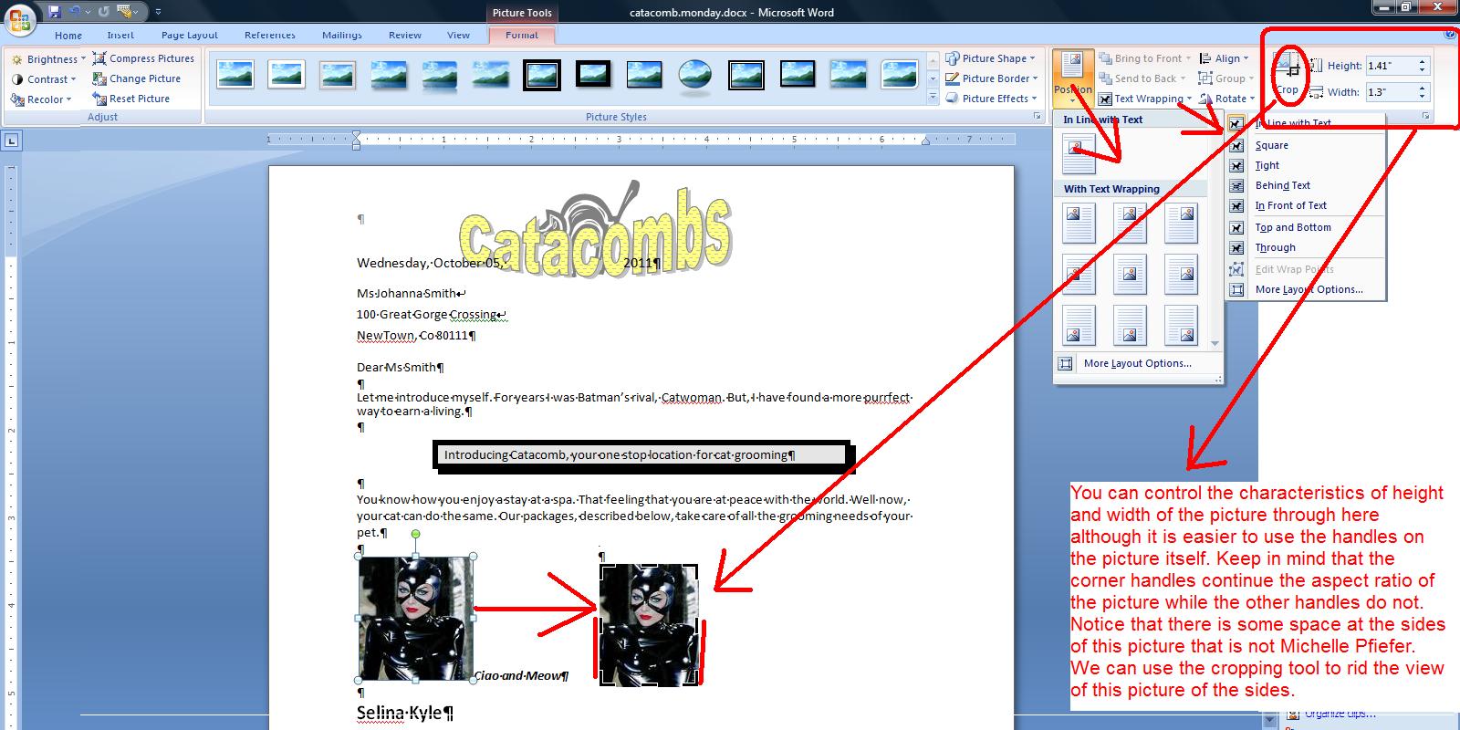
Now, above we have composited this with several features. You can control the sizing of a picture by the use of handles. The easiest thing to remember is that the corner handles keep the aspect ratio (ratio between height and width) while the other handles do not. You can also use the spin controls as indicated top right. The crop control puts a different type of handle on the picture and you can control what sections of the picture should be seen. This is a very powerful editing tool.
We must discuss text wrap. This is the ability of text to manipulate itself around the picture. You can see that when the picture has entered, the text is not wrapping. Two controls handle this. Position which will in essence create a 3 by 3 table around the page and insert the picture intio each cell with the appropriate text wrap being applied. We'll show you this by preview. And, you have the text wrap control whiich applies the text around the picture at the picture's present position.
Several options exist for text wrap. Tight and square are the norms. But ypu also have top and bottom, through, picture above text and picture below text and if we have some time at the end of this problem I will show you these and how they are applied in marketing. For our purposes use tight. Notice also that we have in effect picture styles because we are in native mode. Click a style (I have used an exagerated border) and see what it looks like. Below, you can see what I have done.
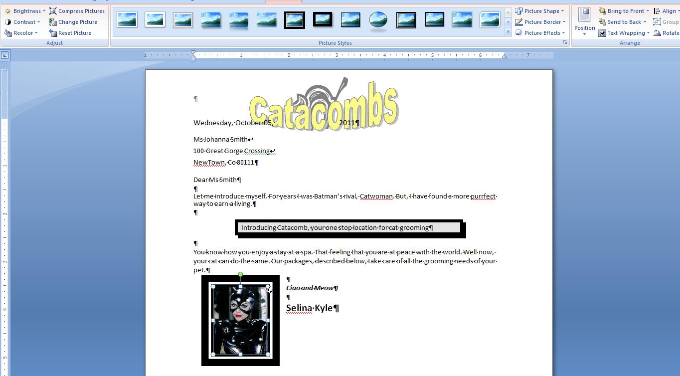
If we have time (and I doubt it) today, let's create the text box at the bottom. Text boxes allow the user to put text (and other things) outside the normal flow of the docment. Keep in mind that you text boes are objects and enter in a similar manner to pictures. You can activate a text box at your mouse cursor by clicking the insert tab and then text box. I am doing this at the bottom of the page.
For those familiar with text boxes there has been changes from the 2004 version. Similar to the templates of header and footer, you now have templates for text boxes. The te,plates will place your text box at specific locations on the page and then, if you want, you can move them. We are going to look at this as the old fashioned text box so click draw text box and with your crosshair create a text box about 5 inches long and 2 inches high at the bottom of the document.
Besides text, you have control of the border and fill per the textbox tools tab that you should be seeing. Type "good for 25% discount at Catacombs" within the text box. On the home tab you have a control Cap A hat. Select this text and click this and the point size will increase. Keep going until Catacombs moves to the next line and then center. Little A hast does the opposite by decreasing point size per what you selected.
Fill and outline of the textbox is on the textbox tool tab in the middle although you can use text box styles for a similar effect. Click outline and then dashes and select a perforated dash. Then select weight and use 1.5 or 2.5 points. For fill, let's use a gradient. After a gradient, which means a change in intensity, chose more gradients and then texture and pick the first texture. Below may be what you are seeing.
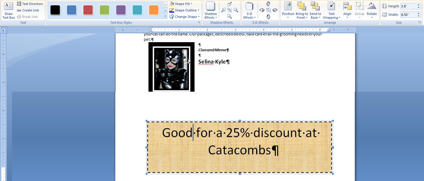
As mentioned in class, we are doing a comparable problem to the Aspen Falls Public Library. You should be doing the Aspen problem on www.myitlabs.com. I believe I have loaded the necessary material onto my course and let me know if this is not the case and we'll add more.
The problem we are doing is slightly harder and moves into the next chapters of the book in terms of tables, quick parts and objects for insertion.
I call this the catacomb(s) problem. Below is a part of what we are aiming at.
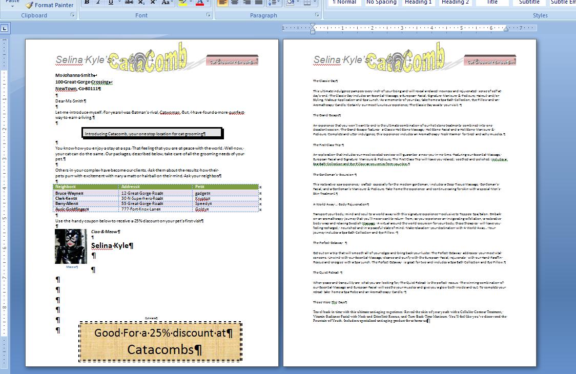
On the Mon-Wed class we had made it to the "let me introduce" paragraph. For Mon-Fri we had only done the address block.
Therefore, if you are in the Mon-Wed class, click here and if you are in the Mon-Fri class, click here
The Mon-Fri group will be putting in the added two paragraphs and I will show the Mon-Wed group the additional capability that Word has added to the mouse.
If you look at the entire document, you are now at the paragraph: Introducing Catacomb, your one step location for Cat grooming. But, it certainly doesn't look like the other paragraphs. it is centered, bordered and shaded.
Your instructor has an interest in how one controls the reader's eyes and this is one trick. Human eyes are attracted to darkness surrounded by light. We will do this with this paragraph. It assures that any eyes that are set on this document will at first go here. The plan is to type in the next 2 paragraphs (introducing and you know how), center the introducing paragraph and then border and shade it. To add effect, we will increase the spacing between it and let me introduce and it and you know how.
Let's discuss justification first. But, to see the full effects, let's work on the You know how paragraph as it has several lines. We had a discussion about word wrap and the process of word wrap autimatically creates a jagged line at the right of the paragraph (assuming left justification). Left justification, the assumption that is automatically made, comes from the characteristics of english which is oriented from the top of the page with paragraphs as left as possible. Other languages (and societies) have other norms.
The picture below shows the 3 paragraphs left justified on the left and right justified on the right. The blue line shows the appropriate margin. The green boxes show the remaining space per line for each paragraph. It is the green boxesthat get manipulated during justification. From left justification to right, the boxes are moved from one side to the other. If we were to center, the green boxes would be split with a half on one side and the other half on the other.
In word, one more justification exits called either justification or full justification. This was made popular by Word perfect in the middle 80's. It is a technique that left justifies while also right justifiying. How can this be done. The green boxes are divided by the number of spaces in the line and added to each of those spaces. This occurs for every line but the last as it would be too obvious in that case. This technique will not work for documents where the average characters per word are high as gaps will be seen. Below, we set these paragraphs to full justification. We have taken the liberty to move lines. At the bottom next to each other is a line form the top paragraph above the bottom paragraph. Look at the spacing indicated by the black lines and circles. You should be able to make out a slight difference in the size of the spacing.
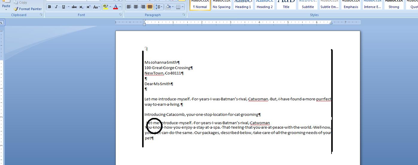
Now having done all this, we would like to center the paragraph starting with introducing. Any changes to the other paragraphs should be undone, You have a tool at the top in the quick access toolbar that is called undo. Another is redo. In word, (and this does not extend to Excel) you can go back and forth pretty much at will. Let's undo the justification changes done to these paragraphs. Below, you can see a composite of what was done. Notice that the undo gives you a detailed listing while redo indicated the next item to redo. The way this works is similar to the use of the navigation keys in browsers in the internet
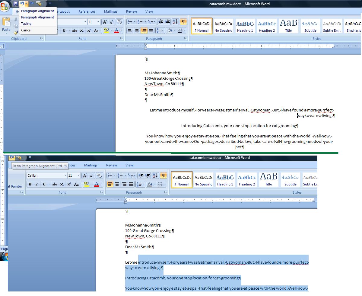
Having done this, let's move to the paragraph starting with introducing. The technique being done could be accomplished with text boxes but we will use paragraph controls. Center this paragraph. Now, move the bottom right control in the paragraph group and click the right portion of the control to see the options. You can see that you can border various parts of the sides of this paragraph. In addition, although we will not use this here, you can set vertical lines which at times is very convenient. We want more, though. Click the last option, Borders and shading and it is here that we will set some aspects of this paragraph.
To the right are various schemes for this bordering. None is an option and disables these borders from being seen. It's the way to turn this off. I normally use shadow, the third scheme for this although you are welcome to experiment. To the right of the type is style color and width. We'll continue with black although feel free to change the color. The style is similar to the underline style we have looked at previously. Choose the first one, a solid line. Width in this case is important. Shadow will not be obvious for width less that 4.5 so click either 4.5 or 6 pts.
You should notice that the preview indicates this shadowing effect. You can deal with each side of the paragraph by clicking it to put it on or off. If you turn on of the sides off, the type of border will be set back to box.
Shading puts a little color (or a gray) into the box You can find this at the shading tab. If using black and white, set fill as no color. In the patterns you will find various possibilities. Ypur audience should determine what percentage to use. If geared to young eyes, head higher. if geared to older eyes, head lower. Keep in mind that your laser printer will probably give you a different effect than what you are seeing. Below, we show a composite of this for you.

Notice that we have the entire line from margin to margin bordered and shaded although the text is centered. To resolve this you can go into the paragraph dialog box and change the paragraph margins or use another technique. First, let's discuss the paragraph margins. This is really dealing with paragraph topography. In many years past, it was common to indent the first line of a paragraph and not space between paragraphs. There is at least one person in this class who learned composition this way. We'll let you decide who is this aged, ancient person among you. As computerization (word processing) made its mark in the 1980's, composition changed. You probably were taught not to indent but to space between paragraphs.
Paragraph topography tries to take this into consideration. Paragraphs are broken down between first lines and all other lines. Firstl ines can be indented or outdented (or as Microsoft calls it, first line and hang). Paragraph margins - called left and right indent - can be applied to all the lines of the paragraph. In the dialog box you see off of the paragraph group are controls to handle all these situations as indicated below.
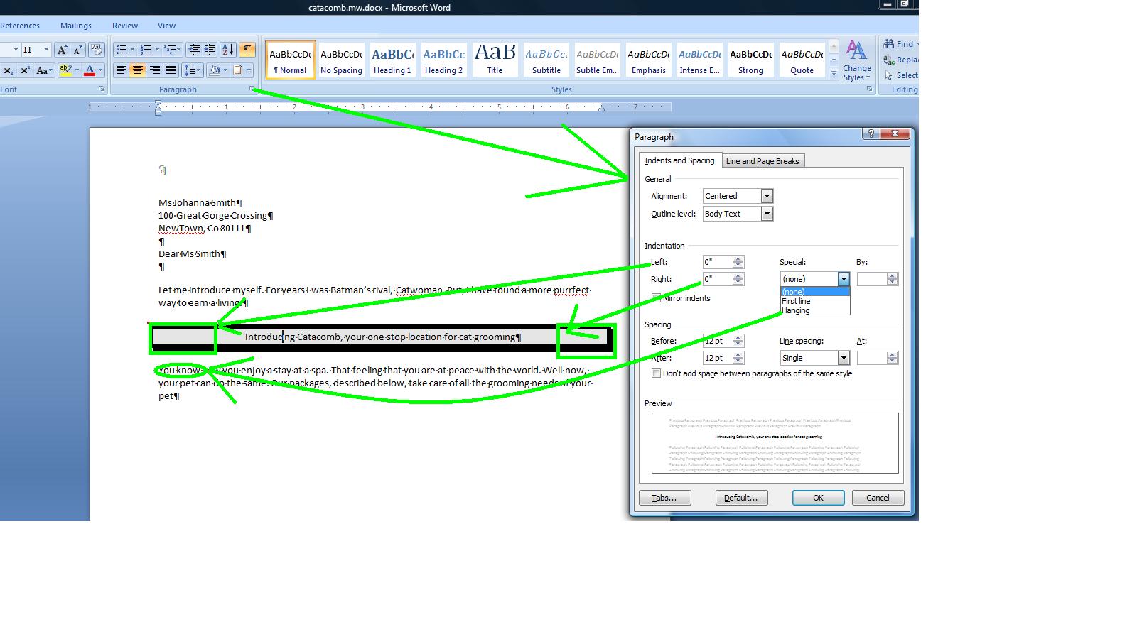
This does seem like overkill to handle this. A better tool exists for this designated as the ruler. Prior to the 2007 version, the ruler was the default. In the 2007 and this version, the ruler starts out hidden. Youi can access the ruler by the control at the right above the right scroll bar or click view and click ruler in the show group. If set on and you get out of the program, the next time Word is launched the ruler will be active. If set off when you get out of the program, the ruler will not show the next time you launch Word.
What does the ruler give you. For any paragraph (or set of paragraphs that are selected) you can control first line or hang, right paragraph margin and the interaction on the left between the first line and the others. Your instructor will show you how this is done on another paragraph and then undo. For the paragraph in question, the omne that is bordered, we need to increase the left and right paragraph margins. Below we see this,
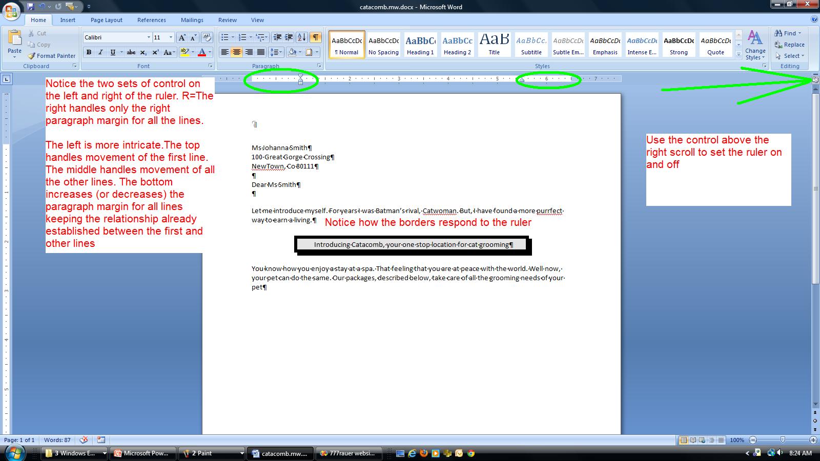
Before heading further down, let's work at the top of the document. Your navigation keys should make some sense now. Use Ctrl Home and you will move to the top of the document in what is designated as the home position of the document. use Ctrl end and you are moving to the end of the document. On any of the paragraphs, use end and you move to the end of that line. Use home and you move back. Sometime in the future we will be using a document that is more extensive and we will have need of page breaks. Move your cursor anywhere in this document and use ctrl enter and you will see a page break created at this point. This is alled a hard page break as you, the user, have created it. Page breaks instituted by the Word program are designated as soft page breaks. By the way, this answers why word wrap points are sometimes designated as soft returns and your enter key is sometimes called a hard return. use your undo to make the page break disappear. Use ctrl home to get to the top of the document.
We want to enter a date as the first line. Hit the enter key to move the address block down further. Now, click the insert tab and click date and time. Dates (and times) can be entered in 2 ways. One is hard wired so that the specific date picked always shows up. The other is by macro, so that the date is picked up from the system and inserted. The update automatically chaeck box handles this for you. The available formats come from the operating system and dates have designation of short, medium and long and you can see this as we have 10/3/11, 10/3/2011,Oct 3, 2011 and Monday, October 3, 2011. Pick the date format you want to show and double click it to insert it. I;ll let you decide whether this is a macro date or specific date.
We would like to handle the header. The 2007 and this version has really changed how Word looks at headers and footers. In a previous class we looked at a predefined header and how it took info from the document properties and used it. Everything is different including how to access the header. You can if you want click the insert tab and then header. It is easier to double click in the header location to invoke this.
When in the header the system helps you with a new tab, the header and footer tool. You can see in this tool a set of control that are of use for the header (and footer). Included are these preset header and footer objects. Date is included as is page number although both of these (you are already aware of date) are in the insert tab options. Access to pictures and clip are also are allowed although again you can use the insert tab of the ribbon for this. Notice that you can also clase the header and this bring you back to the document although it is easier to just double click within the body of the document.
In the Aspen Fall problem, there is a use of clip art in the body of the document. we are going to do the same but just place it into the header instead. We are going to complicate this procedure by intermingling the clip art with word art.
Now, what is word art. It is a cariculture of letters. Below, we track the process of putting a Wrord art object indicating catacomb into the header.
Not shown here is the invokation of an additional tab, designated as Word art tools. If on the word art object, word art tools will show up. if on the header, the header footer tools tab is in operation. Now, on the word art tools, let's look at this. You can space out or compress the letters. You can change the style. In addition you can change the color of the inside (known as a fill) and the outside (known as the border) of the characters. You can even change thei ntrinsic shape of the style although this style was chosen as it looks like a cat as it scratches (you have to be a cat lover to understand this). take a look at text wrapping. When we study picture we will delve into this and positioning more fully but for now, click text wrapping and choose tight. This will move the object somewhat. Move your cursor over calacomb and look for a 4 pointed arrow and when you see it, move the object with your mouse as the left button is depressed. Below, we have put this into position.
Now, back to the header footer tab. Click clip art and a panal will open to your right. Let;s find a cat and so enter cats as the search for. Nothing is more beautiful that jet black cats (in their opinion also) so let's look for a Halloween cat and you can see that I have selected this in the screen shot below.
All right. Similar to the previous object, you have a new tab associated with this clip art (although it will probably say picture). Enter the tab and move to wrap text and set this to tight. Now, move your cursor above one of the four handles at each ofg the corners. You should see a 45% grabber. Move this in till the cat is an eighth of the original size. Move your cursor over the cat un til you see a 4 cornered arrow. Depress your left button of the mouse and move the cat so that it straddles the second C of catacomb as indicated below.
I hope to get to this point in these classes today. If so, we;re done for the day. You can save this if you would like to your flash memory but at our next class there will be a link to load it at that point.
I am going to combine the book's Unit 2 lecture with some things left from Monday. The book is dealing with the Aspen Public Library and you should do the problem in the book. In class, we will do a similar problem designated as Selina Kyle's Cat Emporium.
We start with ewhat is called an address block consisting of name, address, city and state. But before even doing this, let's do some definitions.
A character is a keyboard entry whether you see it or not on the screen and whether it be letter, number or symbol. The space bar is a character although it is used as a delimiter for a word as defined below. You can see every character by clicking the hide show key in the paragraph group as indicated below.
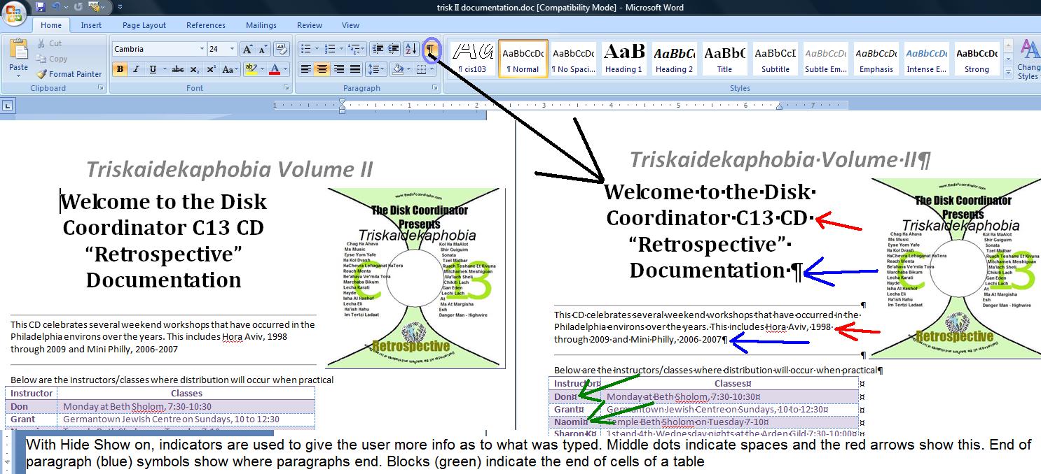
In word processing several characters that are contiguous (together) separated by spaces or punctuation (or the beginning of a document or the end of a document or the beginning of a paragraph or end of a paragraph) is designated as a word. Any word can be selected by a double click on it. FYI: In XP and in Word 2003, there was something called a smart mouse which would automatically highlight the entire word one one of the characters was selected.
A group of words together before and after paragraph breaks (or beginning and end of doucument) is a paragraph. A paragraph break is nothing more than the hitting of the enter key. THius can be selected by a triple click and tyou can see the action as first the word is selected and then the paragraph.
Let's start with a new document. If in Word already, use file/new and select a blank template. If bringing up word without selecting an existing document, Word should put you into a new document.
Notice the title bar up top. The name should indicate Document1 - Microsoft Word. Word defaults to specific names for new possible documents. Documentx where x startts at 1 and increases for every new document added during a launch (launch is a Microsoft expression to designate that a version of word is up and running). You should be in document 1 at this time. You should not save the file with this name and even with the name doc1.docx that the system will substitute when you are in save as.
We have been in Word before. With a blank page, let's determine what Word sets as parameters. First, you should see a blinking indicator at 1 inch down and 1 inch across. This is the I cursor. The I cursor is where you enter text (and objects). Another cursor you should be aware of is the mouse cursor which is free to roam. If we take the serial and parallel discussions from previous classes, the I cursor os serial,the mouse cursor is direct. If I get the chance, I will show you a great new feature that has been added to the interaction of the I and mouse cursor but onward to other things.
2 new definitions. Where your mouse is atv the moment is the home postion of the document. You can always get to the home position by clicking Ctrl Home. As you enter data into the document, the end position of the document moves further down (at the moment with nothing in here, the end position is the same as the home position). You can always get to the end position by the cus of ctrl end.
What about the way this document will appear on the paper. It will not move from the top left of the paper to the bottom right. It is constrained by margins. Because of the nature if printers there is a natural margin of probably about a quarter of an inch. We obviously want to use more than this. Until 2001, Microsoft used the standard of 1" around. In 2001, they changed to 1.25" left and right and 1" top and bottom now known as the Word 2003 standard. For this version, they are back to 1" around. The top and bottom margins are special as they can contain additional information. Margins can be set through the page layout tab and can be changed at any time which means that the program will automatically realign the document as the margin is changed. Below, we show a composite picture dealing with margins.
Not that it means much, but you can also change the size of your paper in page layout under size. In the US there are two standards: 8.5 by 11 and 8.5 by 14. In other countries, however, there are other standards generally smaller than that of the US.
While in this section, we should also indicate that you can change the way the printer prints per orientation. Word (and Microsoft office) supports 2 way: portrait and landscape. Landscape makes you document look as it it has been shifted 90 degrees as it prints.
Let's start with an address block. We will show this to you two ways. One is by traditional paragraphs, the other using breaks. let's start with traditional paragraph ad put your hide/show on.
First paragraph is Mr. Bruce Wayne, second is 1000 Wayne Industry Drive, the third is Bat Cave, NC 28710. Your document should look like:
Mr. Bruce Wayne
1000 Wayne Industry Drive
Bat Cave, NC 28710
and you would see the end of paragraph markers at the end of each line.
We might as well use this for what I was supposed to do at the end of Monday's lecture, a discussion of cut.copy and paste.
To start this discussion, we need to give you even more definition. Word supports character and paragraph commands. In Character commands, you need to highlight those charaters that will be affected. In paragraph commands, you need only select a minimum of characters in the paragraphs you want to affect.
This breaks down into the following: The clipboard and font groups are character commands. The paragraph group is paragraph commands.
C ut, copy and paste therefore are character commands. You already know how to select a word or a paragraph with a double and triple click. How about several paragraphs. You can sweep your mouse through all the text of the paragrapghs. You can use the shift key in conjunction with the directional arrows to select the characters. Or, in this case, since we would be selecting everything in the document, we can use the shortcut of ctrl A. Ctrl A will select everything within a document.
Now, we are in the basis of cut,copy and paste. We might as well use copy. So, click copy in the clipboard group. You may have noticed that the copy icon was grayed out until we highlighted some text. Paste also was grayed out but as soon as the clipboard is activated by a copy or paste, the paste icon is activated.
Below we show this text coppied into several programs: notepad, excel and powerpoint. The clipboard is a system wide resource and can be used anywhere (and in any programs) that support text.

Let's get back to dealing with this document. Supposewe would like to see a different font or point size for this, how and what are we doing. Fonts are styles of characters and the world has plenty of these. You can see these by clicking the top left control in thsi group (it should read calibri) and moving your cursor over several of these selections as was done below. This is preview.
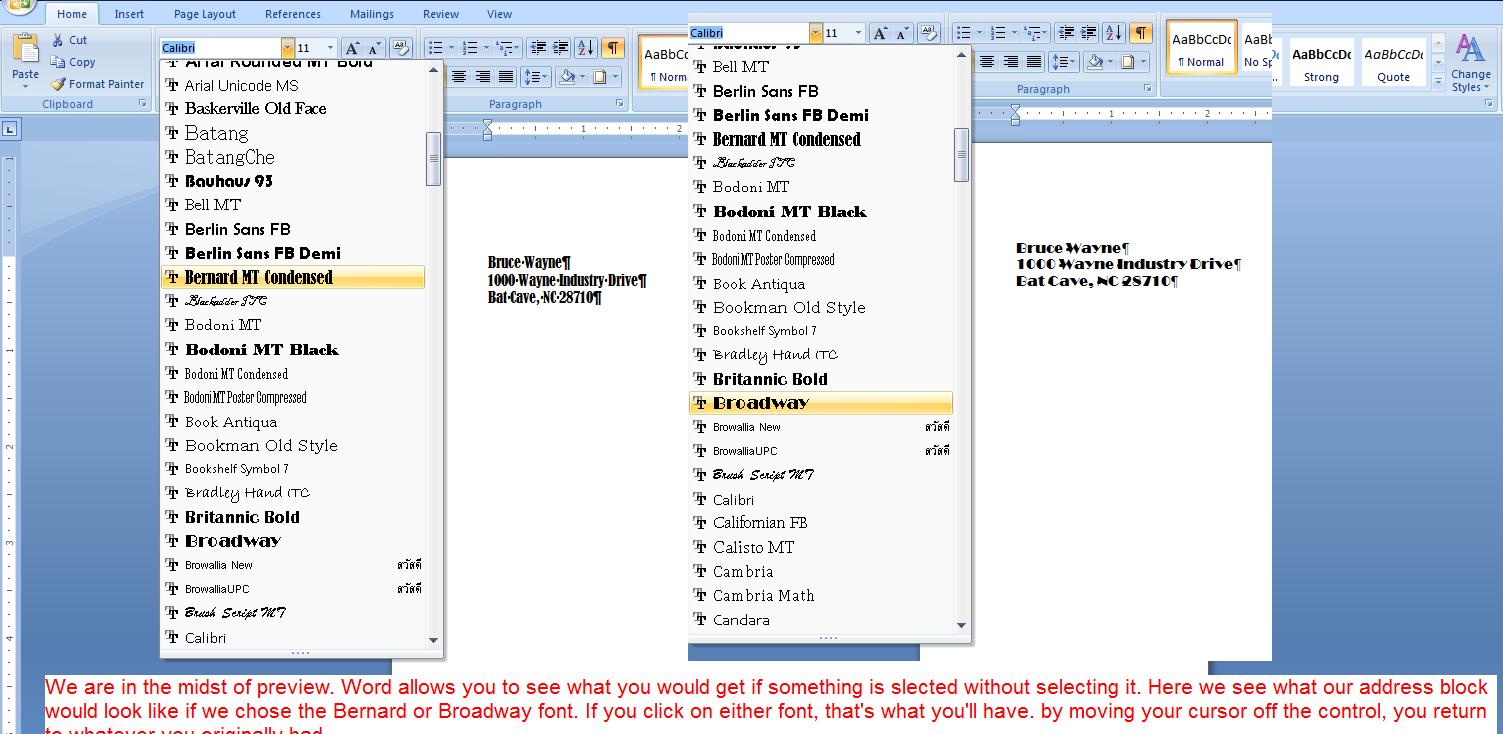
We should mention the use of Calibri. In the 1990 versions of Word the default font was Times Roman, a font created by the Times Of London. Fonts are copyrightable and the use of this font must be paid for. I assume, because of this, the Xp and 2003 versions of Word defaulted to Arial, a font developed by and owned by Microsoft as I understand it. Arial is more open than Timers Roman and probably this is what gave it it's name. Arial 10 was the height of Times Roman 12. For 2007 (and this version) Microsoft has defaulted to Calibri 11, another font owned by Microsoft. Calibri 11 is smaller than Arial 10 (and Times Roman 12).
As to point size, this references the size of the small a in 5terms of the number of periods (dots or points) put on top[ of each other to get to that size. As to displaying point size, it is similar to font and you can preview just as we did for the font. Below, we show this and you should keep in mind that you can preview but without selection the point size will return to what it was before the use of this control
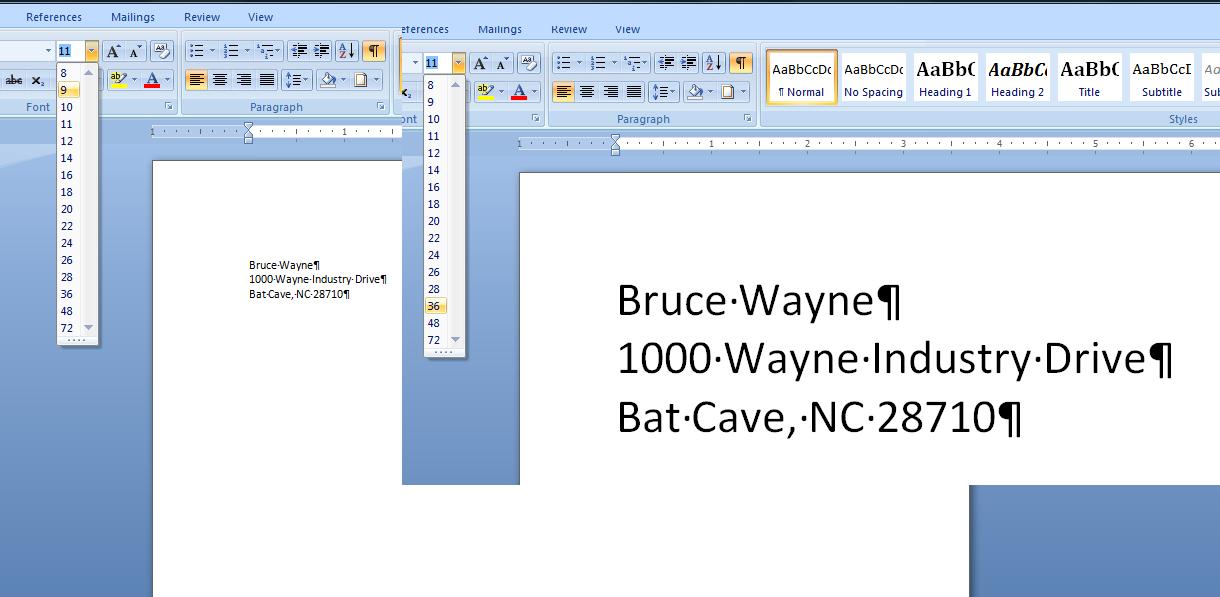
Similarly, you can use preview in terms of underline. The U control in the font group will show a series of underlines when its downward arrow is pressed. Again highlight some text and move your cursor over the possible underlines to see what it will look like. Remember, unless you select, it returns to what it was. Similarly you can do the same thing with colors. In word, there is background and foreground colors,. Foreground id the ink, if you will, and background is the paper. Remeber one rule that every artist knows. A piece of r=text with the same color for background and foreground is invisible,
There are more font controls (and sooner or later we will go over these) but let's concentrate on another aspect of this document now. I need a salutation. After our address block, we want to add Dear Mr Wayne:. This brings up spme problems as to spacing as indicated in the problem in your book. We will discuss several of the possible solutions of your book but understand that we expec t to answer this question with another technique. But first, let's add the salutation. But where?
The traditional way of doing this is to go to the end of the document (the zip code) and hit enter keys as you work your way down the document. In this case, we probably would want to skip a line and then put in the salutation. B ut this version of Word has a better way of doing this. Move your mouse cursor to where you think you would like to add this text beyond the end of the document, Double click and you will find that the system adds blank line (enters, no text) down to your mouse position. In this case, its trivial, but when dealing with a heavy use of objects in addition to text, this technique can save a whole lot of time and trouble. Now, enter the salutation.
After the salutation we need to add another paragraph as indicated below:
Let me introduce myself. For years I was Batman’s rival, Catwoman. But, I have found a more purrfect way to earn a living.
Add this to you document and it should look like the following assuming that we have not changed font, point size, lack of underline and default coloring.
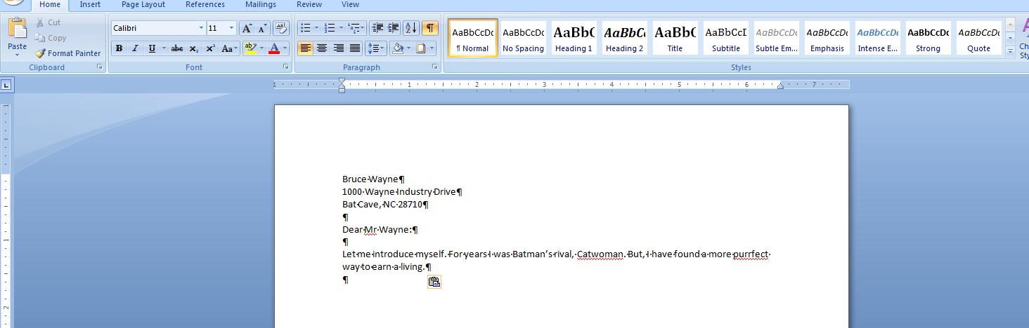
Now, let's discuss this paragraph you put in. Did you specifically create the break between the two lines. We hope not. If you did, you are defeating the entire purpose of this program. The program should have decided when to break based on a whole series of things such as font, point size, margins, etc. The program polls your typing. As you get close to a margin (in this case the right margin) it determines if the word you typed has violated (or encroached) the margin. If it has, it moves that word automatically down the paper to start the next line. We will be discussing spacing and you should understand that what has been defaulted as spacing (or what you have set) determines how far down this next line is. Any changes to any characteristics will force the program to look at your line again. If these new characteristics again have a word encroaching the margin, the line is reset, that word is brought down and it now leads the new line. On the other hand, if added spacing has been created, it will try to fit the first words on the next line up into the end of this line and if it succeeds, the document is completely layed out anew. The word processing industry calls this word wrap.
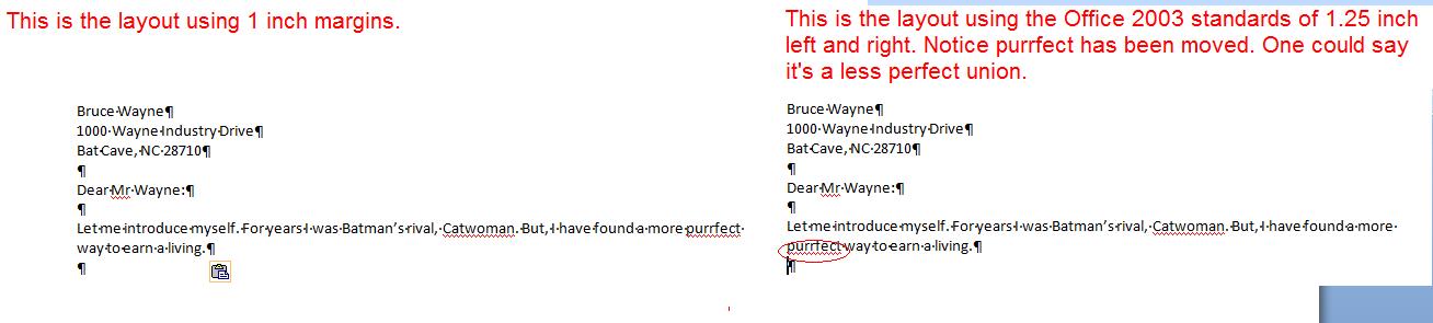
Now, let's look at spacing. There is spacing within the paragraph (between each line). spacing before a paragraph and spacing after. Quite frankly, this is one of the hardest things to control in Word. It is complicated by another factor, the difference in size between the default fonts of 2003 and before and the default font of this and the 2007 version.
Let's take a look at the spacing options. They are part of the paragraph group which should tell you how they can be controlled. Below, is what we would see when this control is pressed. In addition, you can use the dialog box that the group is associated with.
Most of the line options make sense except for 1.15. Can you guess what that might be used for. We'll discuss this in class as we end our lecture
This term we will be dealijng with Word, Excel, Powerpoint and Access. These are part of Microsoft office, one of 11 components. The components do work with each other either explicitly or subtlely. For instance, outlook uses word quite often. But, if you want, you can really get into things as we can show you here. As you will find out, Word does have its own table structure and this is very valuable in word processing. But what if you wanted to load a real excel spread sheet into Word. It can be done as we will show you. Now, interestingly enough, this is beyond what I would teach in Word but we'll do it here to show you the interaction that you can get from these programs and may be something for you to shoot for when you are done studying these application later in the term.
If you have never been in Word before (and the department head assures me that you have), word is domuinated by the ribbon at the top of the screen. Click the insert tab and then click Object and then object again. A series of possibilities should be presented to you, one of which is Microsoft excel worksheet. Click on that and a spreadsheet will appear within your Word document.
Look at the ribbon. When you click within the excel portion, the ribbon looks like excel as you will find out as we discuss excel later in this term. Click outside and you get a perforated type look to Excel and the Word ribbon reappears. This technology, known as object, link and embedding was something Microsoft worked on during the early 90's and Microsoft is very proud of its development of this technology. It still is used today although you don't see and it is hidden within the code of these programs. We are seeing it because we are directly involking it. Below, we show the changes back and forth from excel to word.
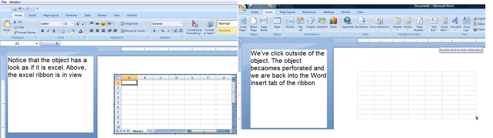
Well. welcome to the world of OLE (pronounced a O-L-E on the East Coast and Olay on the west). Let's do an example of this. Click here to access an access database. In about 7 or 8 weeks you will be able to tell me what is in here. But, till then, I can tell you that there is a table designated as cbl contained within. Let's save this documents.
Now, load up Word and as indicated above, go to the insert tab and click object and access Excel worksheet.
Now, we are about to delve into excel a bit. Again we are about 4 weeks from studying Excel so this may not be clear to most of you. But, you should be able to follow.
In excell, click the data ribbon. TYhis ribbon does have features for accessing what is c alled external data. External data to excel is something that is not resident in a Excel file but is table driven. Database tables meet this criteria. Notice, one of the options is "from access".
Click on "from Access" and drill into the documents section of your machine (or whereever you put the cbl.accdb file). Given that there is only one table in the database, the default will be to access that table and you should see something like what is below.
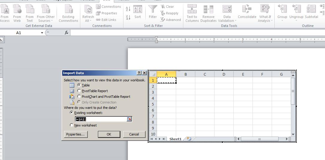
Click okay and the excel sheet, using the access database table info, populates itself. below, is what you should be seeing at this time.
In previous operating system classes, we would use this information to make up an award for the winners of various statistical awards of the CBL but for today we can use this for showing the techniques of OLE.
For your own info, I do believe OLE is used quite often in the underlying coding of the office application programs. Bit, it's hidden from you. Here's an example where OLE is out in the open.
Now, the next thing we want to look at is what can called meta data of a document. For Office 2010, this info can be found in the file tab to the right of the screen under the title, document properties. Below is a composite as we look at Access, Excel and Word's properties.
One of the options is to show the document panel. This panel appears between the ribbon and the document and allows you to enter information about the document. This info is not part of the document, it sts above explaining the document which is why I call it meta info. This meta info can become part of the document by way of the insertions. Let's try this. Click here to load a word document.
Follow your instructor. Use the file tab and info to see the properties. You can keep them up. Now, click on the insert tab and click cover page which you will find out creates a new first page. Click exposure. Now, let's head over to header. Click the header butoon and a series of header templates are shown. Click tiles and below we duplicate this. Notice that info from properties has been added in here.
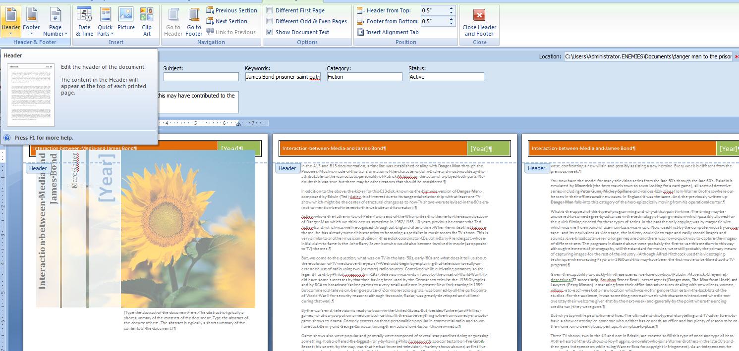
We have used the file tab. let's give you some rules and regulations about file names in Office. You may remember that I said that a file name is made up of a name and extention. Microsoft has had to change the extentions starting with Office 2007. Let's consider Word. The old extention was doc. Today it is docx. What does this mean. When the word program thinks it is running a doc file, it considers itself in compatibility mode. If running a docx file, it is in native mode. Your file above easily shows this. page one has two pictures. You are in native mode. Click a picture and then click the format tab. You should be seeing a set of picture styles on the ribbon.
Now, use file/save as and change your type to a word 97-2003 document and save. This is the DOC type. The format tab should have closed. Open it and the format tab looks different as you are running in compatibility mode. Below we show this.
Let's finish out with one of the oldest Windows technologies, cut copy and paste. In a nut shell, cut deletes the highlighted code. Copy keeps the highlighted code. Paste returns it back to someplce other than the original.
Delete is not a cut. This is a physical deletion. Cut, copy and paste use clipboard mechanism in the Windows operating system. You can see the clipboard in the clipboard group on the home meu in Word and Excel.
Now, you can extend copy and paste. In the document that you have up, highlight a section of code. You can highlight by swiping the mouse or using the shift key in conjunction with the navigation keys on your keyboard.
Click your right button of the mouse and click copy.
This text can be moved thoughout the programs on your system. Launch notepad and click paste. This should appear. Launch Excel and do this also. The text should appear in a cell. Any program with text support should work.
If you want, you can go further. this can be brought back both as text and as a picture. If we have some time, I will show you this feature.
Appendex A of your book deals with several common elements in Office 2010. Today and next Monday we will deal with those topics and some more involving common approaches to the operating system.
Last week we made reference to the fact that several windows applications can be up at one time although please keep in minsd only one of the apps can be the active one. Let's prove this out as far as Office is concerned by loading Word, Excel and Powerpoint onto our system.
Notic, your system should have handled this pretty well. It's a lot of programming and a lot of memory to be used in your system. We have at least 4 things running now, the 3 office apps and the Windows 7 operating system. Can the system run out of memory.
Yes, but probably not. Your computer system uses something designated as virtual memeory to get the added memeory when needed. You can find this virtual memory allocation by following the next two screens.
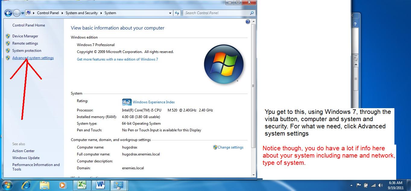
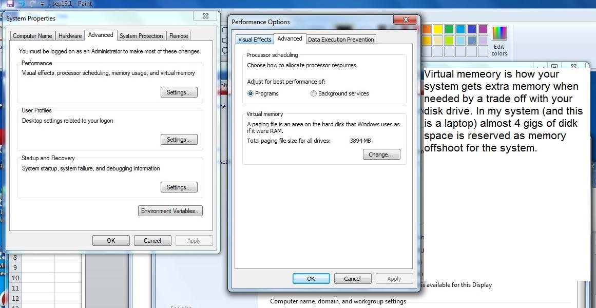
Having seen this now, what is this. It is a trade off with your disk drive. As your system needs more memory, portions of your programs are stored on your disk drive. Other parts of your programs are in memeory and are being executed. Keep in mind that this slows down your machine.
The tip off that your system needs more virtual memeory is the message - system is short of resources, getting more - which occurs when Windows is increasing the allocation of disk space. This is not infinite. Your disk drive is composed of your data and what is needed bby Windows. If you have a full disk drive and the system needs more resources, your system crashes.
Speaking of resources, how can we find out what our system is made up of. Using the accessories portion of your programs, drill down into system tools and then system resources. you will find something similar to below.
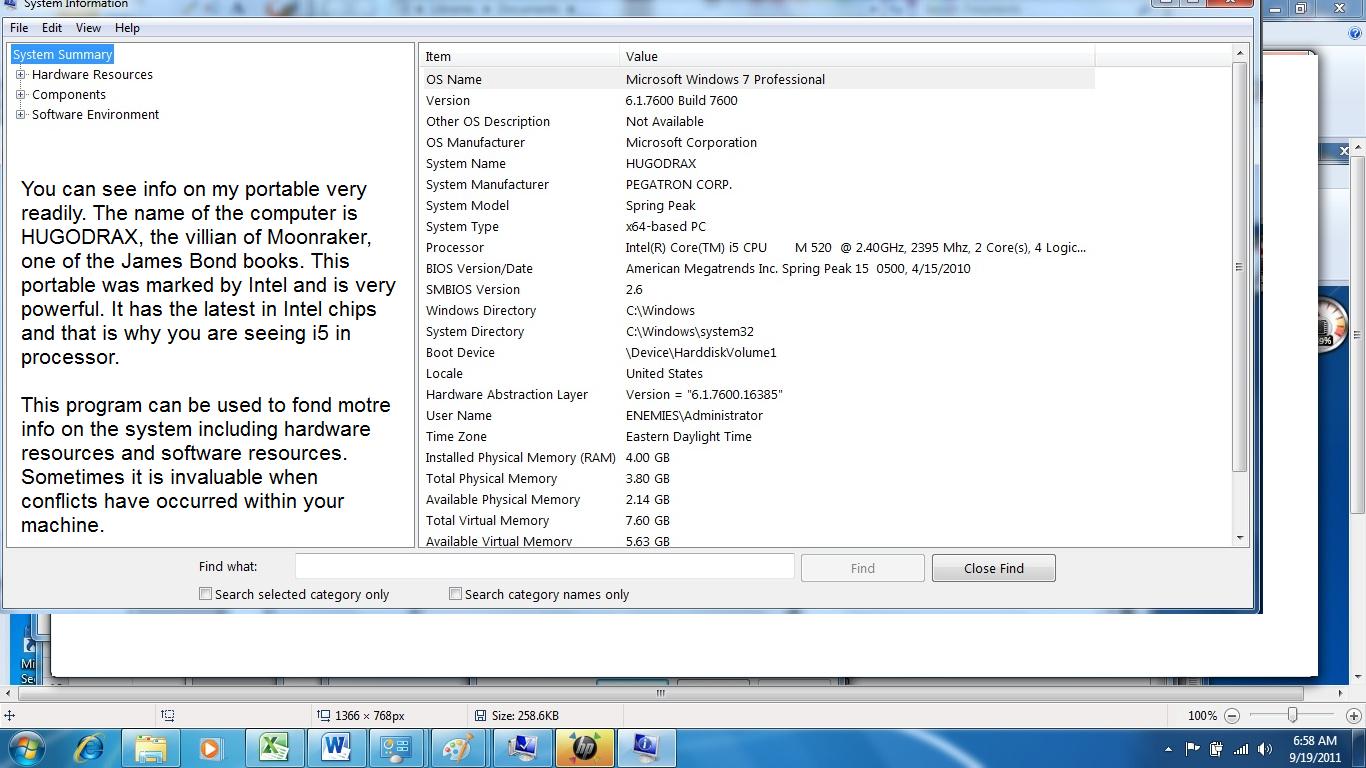
While we are in resources, it wouldn't be a bad idea to discuss a few of these. You have already seen notepad which we used to create our little web page. An addition for Windows 7 is sticky notes. These work somilar to regular sticky notes in real life allowing the user to leave messages for themselves. Below, you can see that I have left messages for myself as to today's lecture.
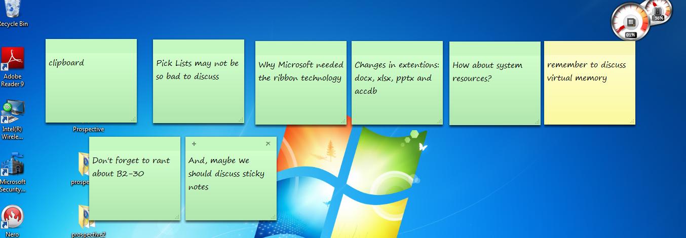
Let's set a few in class. On my system, the first gets turned on by clicking sticky notes on the accessories section. After that, clicking the + symbol creates a clone.
Another nice feature since vista is the snipping tool which can be used to grab info from your screen. Click it and your screen will go whitish. The assumption is that this is a new snip. Use your cursor to highlight a section of the screen. Once completed, the snipping program appears with the screen portion within it and which allows you to save it. Below, I've done the same at home.
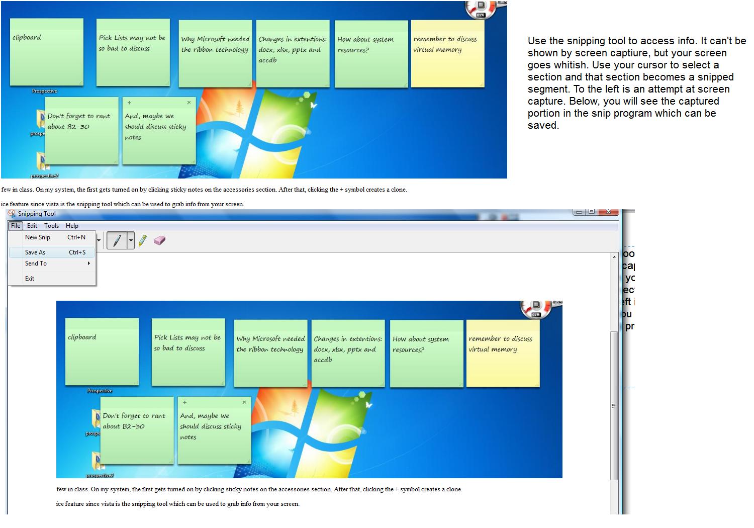
We did bring up Word, Excel and Powerpoint previously. These are part of Microsoft office, one of 11 components. The components do work with each other either explicitly or subtlely. For instance, outlook uses word quite often. But, if you want, you can really get into things as we can show you here. As you will find out, Word does have its own table structure and this is very valuable in word processing. But what if you wanted to load a real excel spread sheet into Word. It can be done as we will show you. Now, interestingly enough, this is beyond what I would teach in Word but we'll do it here to show you the interaction that you can get from these programs and may be something for you to shoot for when you are done studying these application later in the term.
If you have never been in Word before (and the department head assures me that you have), word is domuinated by the ribbon at the top of the screen. Click the insert tab and then click Object and then object again. A series of possibilities should be presented to you, one of which is Microsoft excel worksheet. Click on that and a spreadsheet will appear within your Word document.
Look at the ribbon. When you click within the excel portion, the ribbon looks like excel as you will find out as we discuss excel later in this term. Click outside and you get a perforated type look to Excel and the Word ribbon reappears. This technology, known as object, link and embedding was something Microsoft worked on during the early 90's and Microsoft is very proud of its development of this technology. It still is used today although you don't see and it is hidden within the code of these programs. We are seeing it because we are directly involking it. Below, we show the changes back and forth from excel to word.
Well. welcome to the world of OLE (pronounced a O-L-E on the East Coast and Olay on the west). Again this is somewhat advanced and we won't be studying it but it is a common element throughout office. But so are ribbons. Ribbons were introduced in the 2007 version of office, Prior to that Office used the microsoft memu system. As programs would come up, the menu would play out rigyht to left and clicking each menu item created a panel known as a pop-up menu or context menu. Why switch to ribbon technology and whast does the ribbons give us.
Your instructor can only suspect the reasons. As new features were discussed and scheduled to be added, the menu system and its pop-ups b ecame more unwieldy. In addition, the advent of notebook, laptops, etc changed the screen necessities to a degree.
You are not in for a treat at this point as your instructor will discuss pixels. A pixel is what the system uses as its unit of display. Your screen is made up of rows and columns of these. If you are lucky, your instructor will not mention Philo Farnsworth and potatoes, but Windows requires a certain minimum of pixels to run (800 X 600) while most systems are running much higher in capacity. I do my work on two terminals, one at 1600 X 900, the other at 1680 X 1050. Both of these are 3 times bigger than a window at 800 by 600. What's the effect: Each pixel of 800 by 600 is 3 times bigger than at this higher resolution. HBow does this affect menus. Well, what might seem like a reasonable pop-up menu on a larger resolution system, will run off the screen on the lower.
Microsoft's ribbon technology handles this. Each tab of the ribbon is made up of groups. The groups are programed to display either horizontally or vertically given the resolution of the screen. It also will compress and decompress components as the need arises. Below, we show the ribbon in several resolutions.
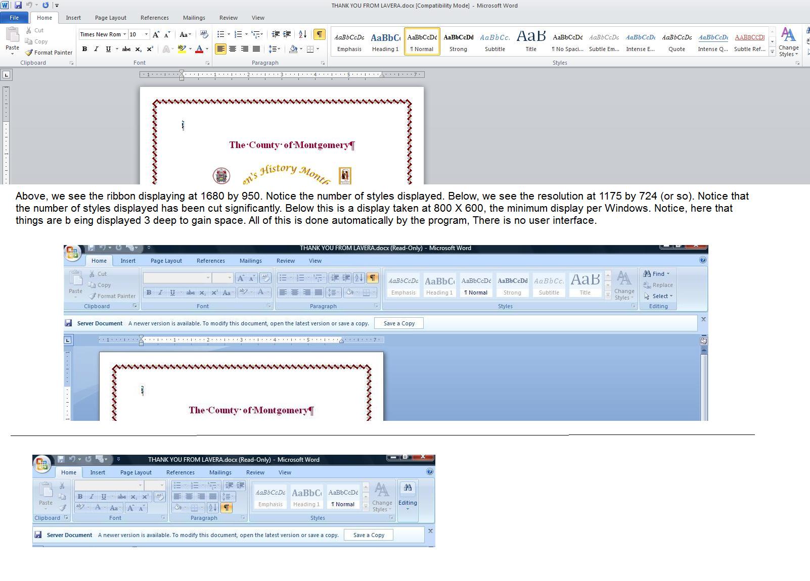
We already told you that there are pictures of each class. TYhey can be accessed through here. For informal pages such as ours, the size really has no meaning but on web pages that are quite extensive, this could be an issue which we will discuss. Anyway, here are the pictures in jpg format.
For the wed class, wed class 1 and wed class 2
For the Fri class, Fri class 1 and fri class 2
Let's start with the pictures. A Picture, as will be a word document, as will be an excel spreadsheet is generically designated as a file. It wasn't always the case but today the type of file this is is designated by the extension. File names are set as name [.] ext. Take the case of fri class1.jpg (one of the file names). fri class1 is the name, jpg is the extension. Your operating system is keyed to extensions and the operating system keeps a list of programs that work with this extension. Microsoft calls this 'documentcentric'
FYI: Jpg is just one of several extensions that the system recognizes as a picture. Other extensions are jpeg, gif, pnp (and others).
Having this picture on the web won't help us as far building the little web script is concerned. There are several ways to save a picture. When up in the browse, move your cursor over it and click your right mouse button. One of the options is save as. In addition, you could have moved to the file menu tab at the top, clicked that and used save page as to get the same result. Below we show this as a composite.
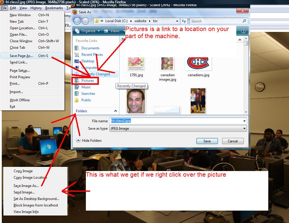
But we are a little bit ahead here. Where do we save these pictures both in a generic way and a specific way.
Files (which includes pictures) cannot sit alone. They are stored on folders - or if you are as old as yuor instructor - directories. A directory can hold multiple files. The directory has a name and in this operating system, the way to access this file is folder\name of file. As an example, let's assume we have the pictures folder and have saved fri class1.jpg into it, accessing of this jpg file would be pictures\fri class1.jpg.
Now, you may not be aware of this based on the fact that over the years MIcrosoft has developed some shortcuts to access different folders. And the different folders pertain to your identity on the computer system you are using. This is what is studied in a computer class dedicated to learning about operating systems. This is not that class so I will show you a little about this on the screen, but we can't use what you would normally expect from commercial software which is set to automatically aim at these locations. We are going ot be writing a free scripted program using notepad which does not provide these links. Below, only for your info is how your machine is organized. This is much to complicated to try to decipher for what we are doing.
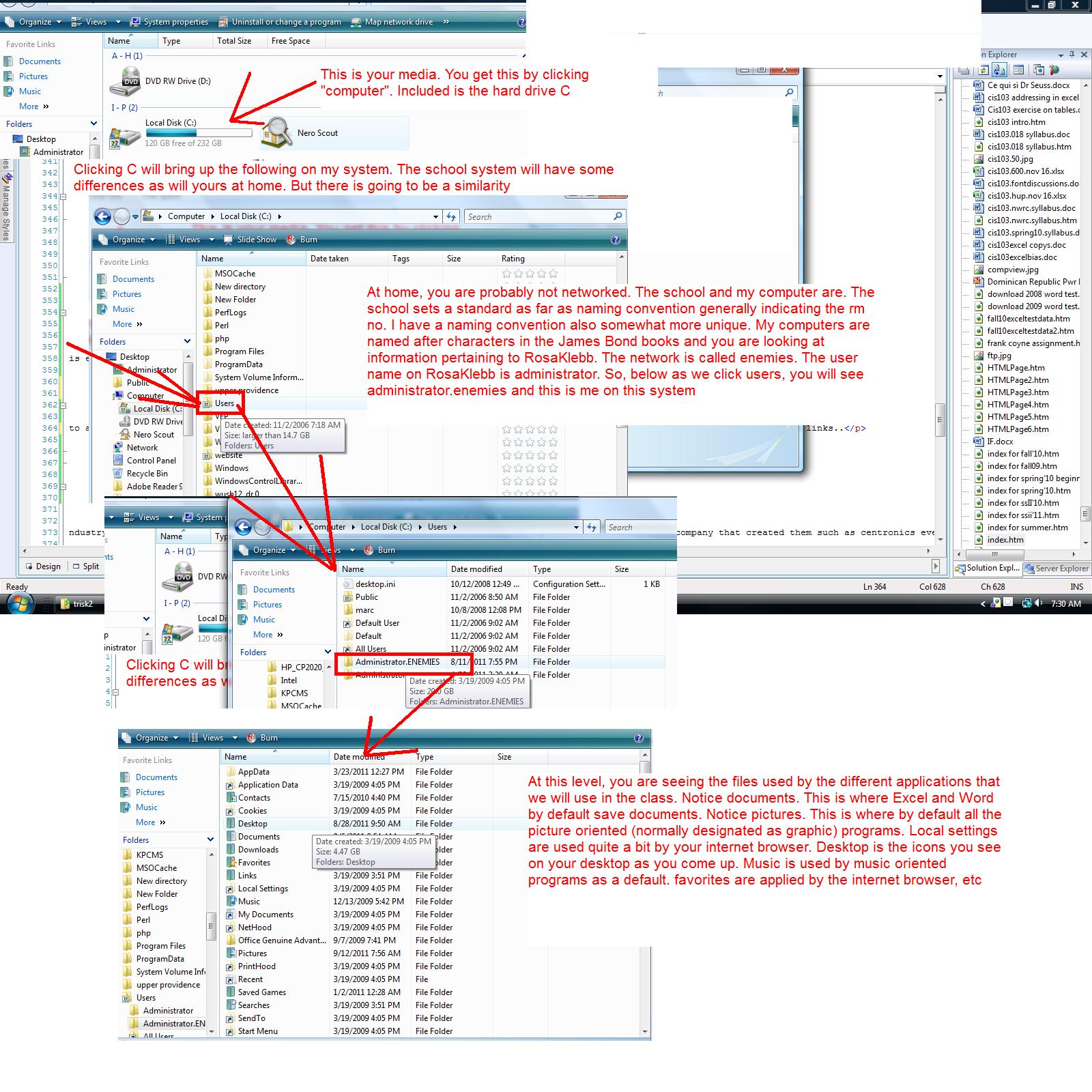
So, what are we going to use in class to save our picture files. We are going to create a new folder/directory off of the C drive. We will call this new folder, class. Now, to do this, understand that the operating system gives you an option of new when your cursor is placed correctly over a folder. By correctly, I mean over the white space (or blue space) and not any of the objects. By clicking your right button, you will see the "new" option. Clicking new gives other choices but at the top is new folder. When this is clicked, a new folder icon will show up and will expect you to type a name. For this folder, we will call it class as mentioned before. Below, we show this.
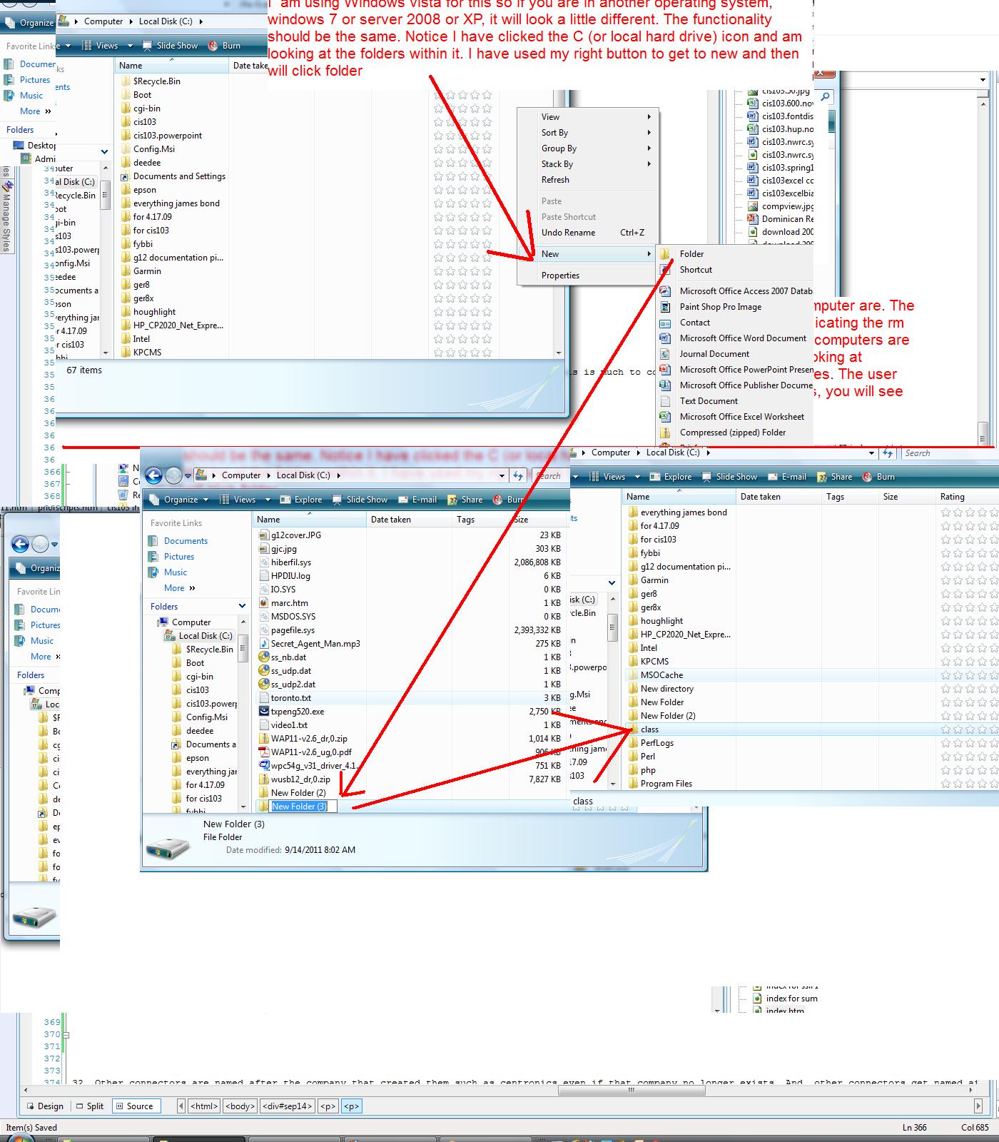
we will use the folder class to hold our pictures. The official address of this folder is c:\class (although when setting this up in HTML, we can use c:/class). Any picture in it, like fri class1.jpg would be referenc3ed as c:\class\fri class1.jpg
Now, let's access the two pictures pertaining to the specific class and save these into the class folder. Similar to what we have been doing, we should be able to see this using the file structure. Again, click on computer and the C drive. Class should be a folder and click on that to see what is below.
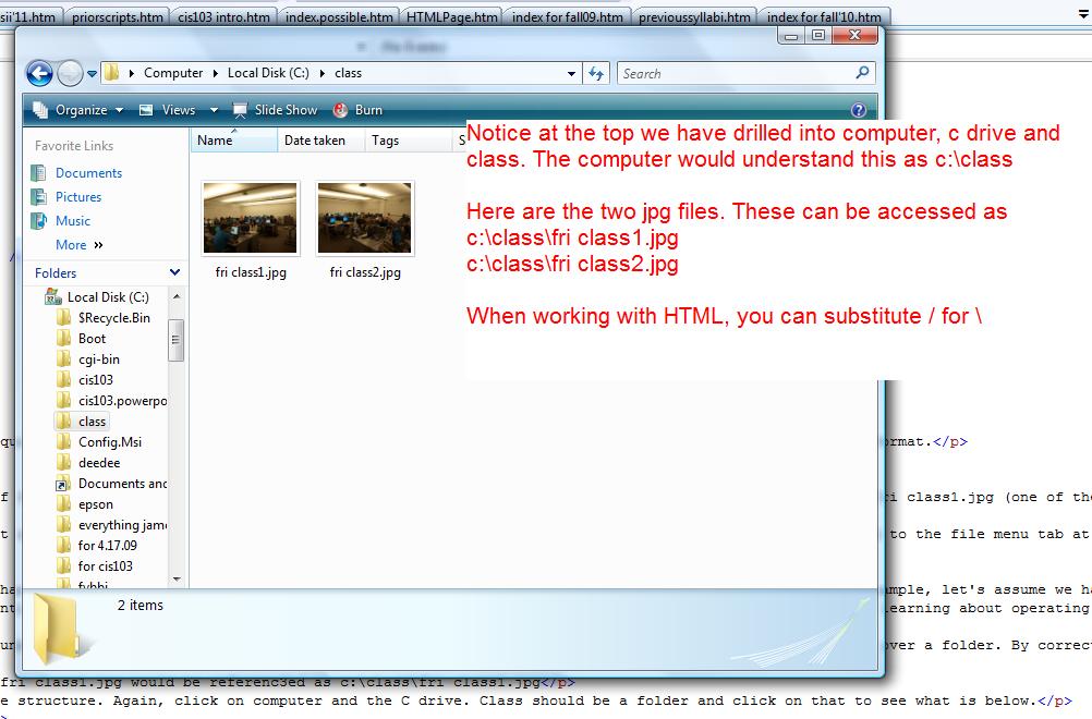
Now, similar to the pictures, we need a location to save our HTML file. HTML files have the extension htm or html. We might as well use the class folder. We will save changes to the HTML file into this folder. To create and change this html file, we will go back into technology and pull up a lowly text editor called notepad. Now, before we talk about how to do this, text editor as what you type is what you get. No additional code is created in the file. All the other MIcrosfot applications we will use are what you see is what you get. A considerable amount of hidden code is added to these. So, if you try to duplicate this at home, you cannot use a word processor or desktop publisher. The additional coding created by these programs would mystify your browsers for the most part (although sometime it will work). Notepad can be found under programs and then accessories as indicated below as I bring it up on my system.
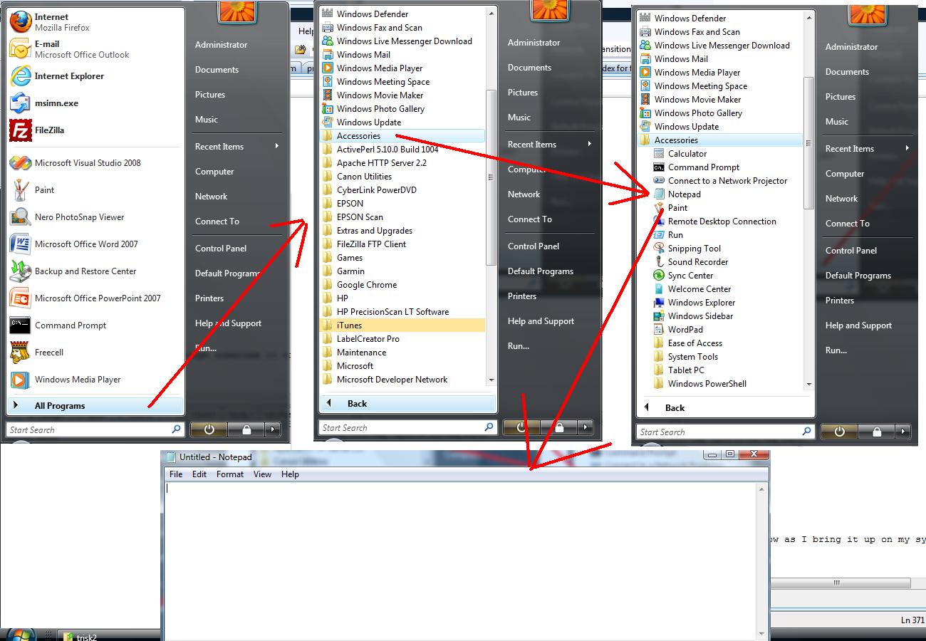
Now, we are going to deal with two programs and if you want to make this easy, keep both up on your desktop. One of these programs is notepad, the other is any browser and for this class let's use Internet explorer. While notepad is up, click to bring up Internet explorer. You are now looking at two windows. The window that is active is not truncated and its title is a full color. A window that is not active may be truncated or overwritten and its title is grayed out. If overwritten, as in this case, you can control this by the icons at the bottom. Below we see an example of this.
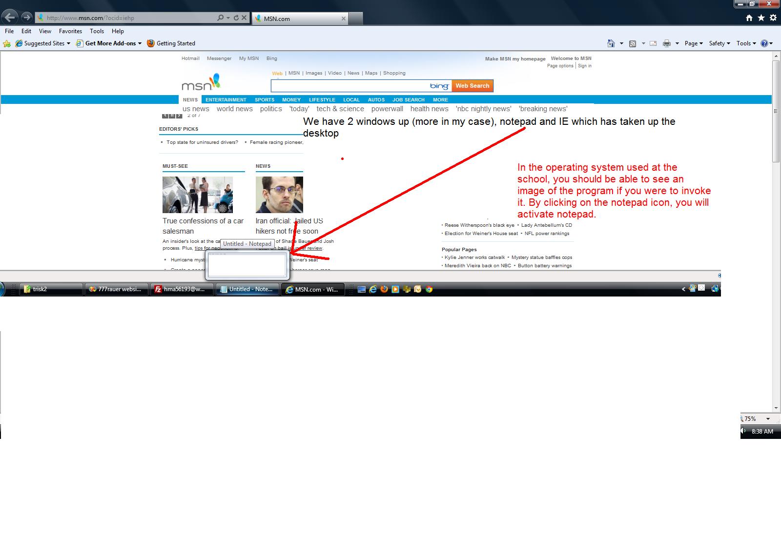
Now, activate Notepad and type in the following:
<html>
    <head>
        <title>[my] web page</title>
    </head>
    <body>
    </body>
</html>
Now we need to save this and we need a unique file name. Let's use cis103.htm. Click save. Below shows this.
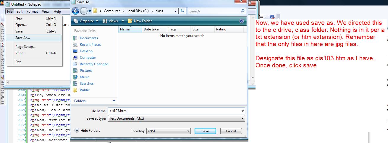
Now, bring up Internet explorer. Type in at the URL locator, c:/class. At this point you should see toips that include cis103.htm. Click that and you will see title. Below is an example.
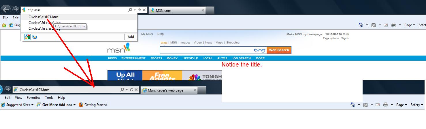
Let's add some other things to this in the body. The P tag stands for paragraph. There are variations of this in cluding the H tags which I may have obsessed upon in one class. We will work with the p tag. We want to print out: This is my class in computer technologies at CCP. Now, inadditon, we want to show one of the pictures. This is the image tag using img as the designation. You add the source of the file that is the picture to this. so you would see img src="c:/class/friday class1.jpg" with the less than and greater than brackets. Finally, let's separate this by adding a line across the bottom. In the end our code looks like:
<html>
    <head>
        <title>[my] web page</title>
    </head>
    <body>
        <p>This is my class in computer technologies at CCP.</p>
        <img src="c:\class\fri class1.jpg">
        <hr>
    </body>
</html>
Now, we want to do this smartly. Your notebook file is still open, down at the bottom somewhere. Click to maximize. Put in the added code. Now, click file save. Minimize if you wamnt, but do not close this. Now, go into IE. Hot f5 or Ctrl f5. You will see that the body now exists.
We do have a problem. The picture is too big. There is attributes of various kinds that you can use to control things. We are going to use more modern techniques. This involves CSS (cascading style sheets).
Tghe general form of this is style="xxxxxx:yyyyyy;zzzzz:aaaaa". In the img tag, put style="width:25%". This should limit the size of the picture to one quarter the size of the screen.
However, let's add to the point size of the text. Add thsi attribute to the p command: style="font-size:150%". On the hr (which you see is not printing, let's add style="border-style:solid". This should look like:
<html>
    <head>
        <title>[my] web page</title>
    </head>
    <body>
        <p style="font-size:150%">This is my class in computer technologies at CCP.</p>
        <img src="c:\class\fri class1.jpg" style="width:25%">
        <hr style="border-style:solid">
    </body>
</html>
While I interchanged the image and the hr, you can see what I got below.
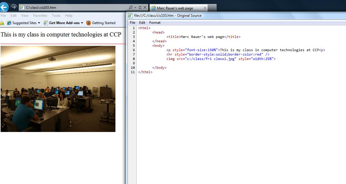
Now, finally, one of the powerful features of the Internet is it's ability to link to other sites. This is accomplished with the where to click tag. If linking to a web page site, we have to give the official hypertext link. So, for instance, if trying to link to the school's page, we would use http://www,ccp.edu. In the a tag, you use the attribute href= to direct the system to the next site.
Putting all this tigether, our command would look like <a href="http://www.ccp.edu">Click here to go to the Community web site </a> and adding this to our code we get:
<html>
    <head>
        <title>[my] web page</title>
    </head>
    <body>
        <p style="font-size:150%">This is my class in computer technologies at CCP.</p>
        <img src="c:\class\fri class1.jpg" style="width:25%">
        <hr style="border-style:solid">
        <hr>
        <a href="http://www.ccp.edu">Click here to go to the Community web site </a>
    </body>
</html>
And below we show the web page. Clicking the underlined code (designated as a link) will send us to the school's web site.
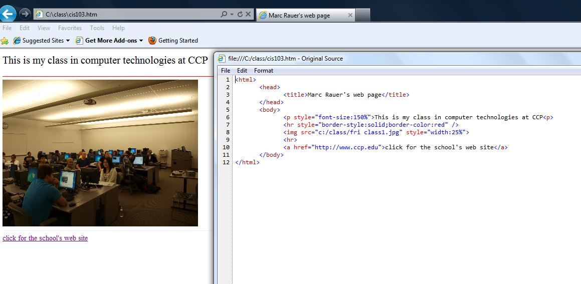
For one of the classes, we discussed the types of connections in computer systems. You can read about this in the data communications section of your book (blue pages, chapter 12)/
Computer engineers over the years have come up with two ways of communicating data, Asynchronous (known as serial) and Bisychronous (parallel) over the years. Serial, by far and away, is the most common way of transmitting. Parallel is used most frequently with printers.
Your computer has ports for handling the transmission of data to and from your machine. In the old days, specific connections (and connectors) were used. Your book has pictures of these connectors with the cables. Connectors are the term used for the individual hooking up parts of the cable. It used to be that established connectors from other industries would have designated terms such as type A and this would be used. New types that were created specifically for the computer industry might get terminology pertaining to pin structure such as RS 232. Other connectors are named after the company that created them such as centronics even if that company no longer exists, And, other connectors get named after the underlying technology that they are invoking such as vga.
Everything moves in and out of the chip through the board to your periferals by way of serial or parallel transfer. Inside the case, this is the realm of the service technician and the computer engineer. Once it get's to your case, it becomes your porblem in how to control this.
To make it easier for everybody, a new type of connector was introduced in 1996 or so designated as USB which could be either serial or parallel depending on what was the usage.
Now, again, let's delve a little bit further into the concept of serail and parallel. Serial for the most part is one way. Look at it as a one way street. In general things go one way down the street. It's only when everyone agrees that movement can go the other way that we can violate the one way nature of the strret.
Parallel acts as a two way street so that information is flowing the other way even as info moves the other way.
Keep in mind that many of these concepts are being developed when computer equipment (and maybe equipment in general) is in its infancy so it is possible that today, if this was reinvented, something different might have been used and designated.
Let's discuss parallel. In printing, you cannot print while the printer has certain problems such as a jam, paper out, toner out, etc. In the old days, you had to have someway of telling the computer to stop sending info to the printer. Here's where parallel would play its role by getting feedback immediately and then stopping the process until the problem was cleared.
Now, we should add that serial has its own checks but these are done after the fact. A lot of data is transmitted through the connection. That data is, in essence, made up of 1's and 0's. A check sum piece of info is send at the end of the transmission. The check sum could be as easy as the sum of bits that are on (the 1's) mod 256 (the remainder when a number is divided by 256), Each side of the transmission is doing it's own math while the information is being send, The sending component sends this info at the end of what is known as a stream and the receiving part compares. For this small time it is agreed that no transmission will be occuring in the normal direction. This opens up the possibility of communications in the other direction and the receiving component sends a message to the sending componebt whether the check sum is legitamate. If so, the next set of data is moved through the line. If not, the sender repeats what was sent before.
This discussion, which your instrcutor will touch on, can be extended into protocols. Generally in sending info the type is known (serail or parallel). The protocol stands for how the info will be configured and in Internet transmissions a protocol TCP/IP is used throughout the world. One other factor is called blocking. This is combining several packets of a protocol together on a transmission and you do this when communicating with your ISP.
Now, having discussed communication in some way, let's move to the next discussion. In one of the classes, I brought down the pictures I had taken on the class. In the other, on Friday, I did not get to that point. For the 11Am class, we will bring down the video today so you can see this in operation.
Digital still and video cameras today are like small computers and use USB connections to download pictures. We will discuss what a picture is, but dealing with transmission it should be clear that with the media involved, we can use serial transmission with, no doubt, several check sum checks to make sure the transmission is really accurate.
Now, let's access the picutes.
For the wed class, wed class 1 and wed class 2
For the Fri class, Fri class 1 and fri class 2
we are aiming at doing a small web page. We'll use these pictures, a little text and a link to the school's web site at www.ccp.edu. This is not a unique type web site - there are perhaps a billion of these, literally, in the world today. First, though, we need to deal with the pictures.
Your operating system has a location reserved for pictures called pictures, interesting enough. Below, I have moved my cursor over the picture, clicked the right button and selected save to file. You can see what we have at that point, below. I choose pictures if that is not already the option and save.
Before studying the picture, what is a program? Remember the chip. The chip has specific "machine language" instructions. A program is made up of machine language instructions that tell your chip what to do to resolve an issue. It is very specific as far as instructions. We deal with programs all the time. All the components of Ofiice 2010 are such programs.
There are many picture editors in the world. From Microsoft you have the old standby, Paint, which is what I use. You have the Windows photo gallery that comes with all operating systems since Vista. And Picture viewer which comes from Microsoft Office. Go into the pictures folder and move your cursor above a picture. If you double click at this point you will execute a default program your operating systen has set for these types of files. If you cvlick on your right button, you will get some options including open with. This is an attempt by your operating system to indicate additional programs you might want to use. Below, we see this on my system.
Let's use picture viewer if it exists on your system and bring this up or windows photo gallery. Each of these programs have different tools with pholo gallery having more controls. We can play with some of the controls to show you how these work. Notice that nothing seems to be wrong as far as size.
Now, let's go back and look at this through Paint. Seem slightly different? Below should be similar to wwhat you are looking at!
We mention this because internet technology resolves this and you are seeing that in Windows photo gallery. It has already reduced the picture. But, keep in mind that if using this on something that is to be transmitted, the full size is used and this could slow down what you call the speed of the internet.
Below, is the lecture used during the summer for a little web page. I;ll duplicate this here althugh there will be changes in terms of what we are doing.
We start the simplest web page by the following commands.
<HTML>
    <head>
        <title>[my] first web page
        </title>
    </head>
    <body>
    </body>
</HTML>
 Let's put this into notepad. You can find notepad off your start button under accessories. it should look like whats to the right.
Let's save this. We'll use your name. The extension should be htm. If it's me, I'm looking at marc.htm.
Now, several things about this. Caps or non caps are allowed. I could do MaRc.HtM and get the same result.
the extension htm ties this to an internet browser, probably Internet Explorer on the school's computers. We will use this feature by just clicking this file when it is saved.
Where do we save it. Anywhere really on the disk as long as we can remember where it is. The school's computers run on XP so we should be able to access the root directory of the c drive. We should be able to get away with c:\marc.htm (and yes, this is a back slash which you can find below the question mark.
Below is a view of the root directory of my computer. Since this machine is using Microsoft Vista, it will look different from what you are seeing although I will be walking around to make sure you are set correctly

Now double click this entry. This is using what Microsoft calls the documentcentric nature of the operating system. The system checks the extension and then finds the program associated with that extension. The program is brought up and then loads this file. On my machine, Firefox is the default for htm. On your machine at the achool, Internet Explorer is probably the default. Wichever, a browser will be launched and you will see your script being run.
First: look at the top. Your title should be displayed. Second, click view/source and you will see a replay of what was typed. Below we see this.

Let's continue. Move back into Nopepad. The next HTML instrcutoon (known as tags) is the p command which really means paragraph. Assume we wanted to display the following text: What I did on my summer vacation? I created this web page.
Between body and /body we would put the following command:
<p>What I did on my summer vacation? I created this web page</p>
:et's add this to our notepad file. Now, don't forget to save the file with these changes. Move back to the browser and hit the ctrl key in conjunction with the f5 key. Ctrl f5 should reinitialize your browser and display the page again with the new code.
What if we want to center the code? We have choices. The easiest is the html center tage put in front of the p tag and having a /center put after the /p. You can do something called CSS operations. For our purpose here, let's use center. Here's how the code changes:
<center><p>What I did on my summer vacation? I created this web page</p></center>
Below is what this should look like
We want to add a picture. Pictures are the forte of HTML. If there was no need for pictures, the internet as we know it wouldn't exist. The template for a picture insertion is to use the img command. here's what it looks like:
<img src="[file structure location of picture to be inserted]" >
It becomes difficult to show this accurately because of the file structure difference between vista and xp so we will continue in detail on the board
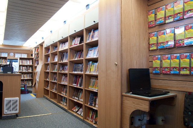
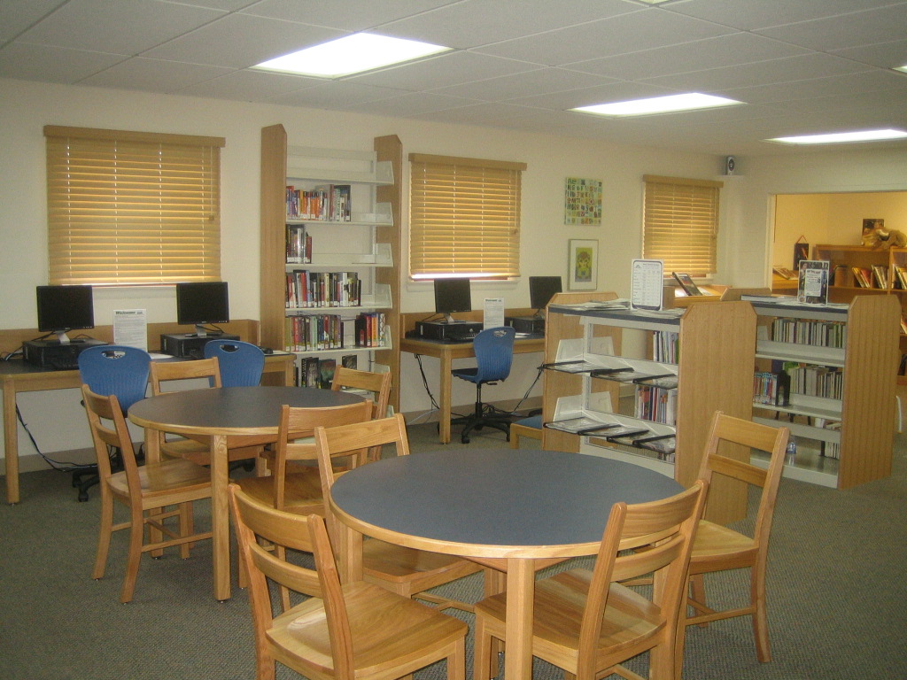
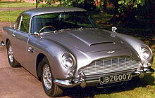
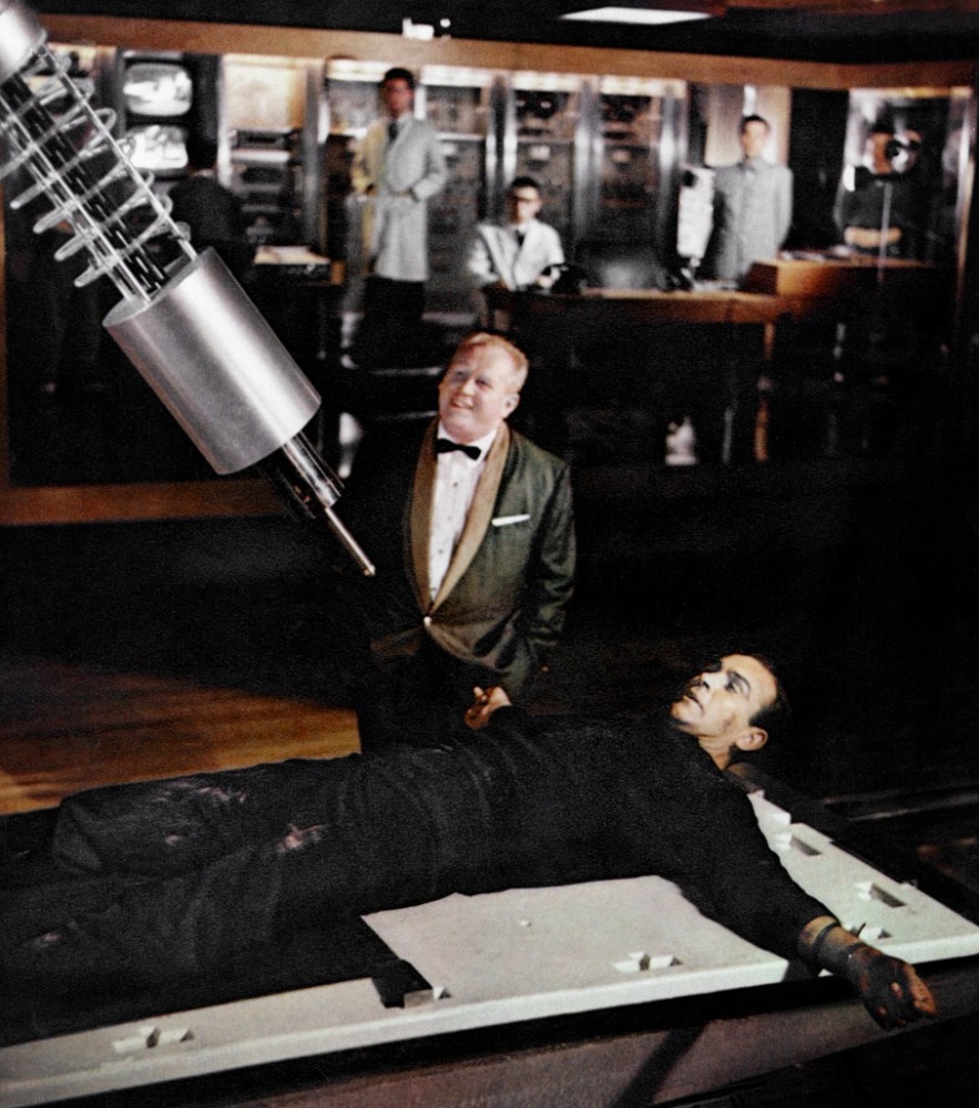